Threshold Choice Methods: the Missing Link

Jos´ e Hern´ andez-Orallo Departament de Sistemes Inform` atics i Computaci´ o Universitat Polit` ecnica de Val` encia, Spain

Peter Flach Intelligent Systems Laboratory University of Bristol, United Kingdom

C` esar Ferri

Departament de Sistemes Inform` atics i Computaci´ o

Universitat Polit`

ecnica de Val` encia, Spain

October 26, 2018

Abstract

Many performance metrics have been introduced in the literature for the evaluation of classification performance, each of them with different origins and areas of application. These metrics include accuracy, macro-accuracy, area under the ROC curve or the ROC convex hull, the mean absolute error and the Brier score or mean squared error (with its decomposition into refinement and calibration). One way of understanding the relation among these metrics is by means of variable operating conditions (in the form of misclassification costs and/or class distributions). Thus, a metric may correspond to some expected loss over different operating conditions. One dimension for the analysis has been the distribution for this range of operating conditions, leading to some important connections in the area of proper scoring rules. We demonstrate in this paper that there is an equally important dimension which has so far not received attention in the analysis of performance metrics. This new dimension is given by the decision rule, which is typically implemented as a threshold choice method when using scoring models. In this paper, we explore many old and new threshold choice methods: fixed, score-uniform, score-driven, ratedriven and optimal, among others. By calculating the expected loss obtained with these threshold choice methods for a uniform range of operating conditions we give clear interpretations of the 0-1 loss, the absolute error, the Brier score, the AUC and the refinement loss respectively. Our analysis provides a comprehensive view of performance metrics as well as a systematic approach to loss minimisation which can be summarised as follows: given a model, apply the threshold choice methods that correspond with the available information about the operating condition, and compare their expected losses. In order to assist in this procedure we also derive several connections between the aforementioned performance metrics, and we highlight the role of calibration in choosing the threshold choice method.

Keywords: Classification performance metrics, Cost-sensitive Evaluation, Operating Condition, Brier Score, Area Under the ROC Curve ( AUC ), Calibration Loss, Refinement Loss.

([email protected])

([email protected])

([email protected])

Contents

1 Introduction			2
	1.1	Contributions and structure of the paper . . . . . . . . . . . . .	5
2	Background		6
	2.1	Notation and basic definitions . . . . . . . . . . . . . . . . . .	7
	2.2	Operating conditions and expected loss . . . . . . . . . . . . .	7
3	Expected loss for fixed-threshold classifiers		9
4	Threshold choice methods using scores		11
	4.1	The score-uniform threshold choice method leads to MAE . . .	12
	4.2	The score-driven threshold choice method leads to the Brier score	13
5	Threshold choice methods using rates		15
	5.1	The rate-uniform threshold choice method leads to AUC . . . .	16
	5.2	The rate-driven threshold choice method leads to AUC . . . . .	18
6	The optimal threshold choice method		20
	6.1	Convexification . . . . . . . . . . . . . . . . . . . . . . . . . .	20
	6.2	The optimal threshold choice method leads to refinement loss . .	22
7	Relating performance metrics		24
	7.1	Evenly-spaced scores. Relating Brier score, MAE and AUC . . .	25
	7.2	Perfectly-calibrated scores. Relating BS , CL and RL . . . . . . .	26
	7.3	Choosing a threshold choice method . . . . . . . . . . . . . . .	30
8	Discussion		32
	8.1	Related work . . . . . . . . . . . . . . . . . . . . . . . . . . .	32
	8.2	Conclusions and future work . . . . . . . . . . . . . . . . . . .	33
A	Appendix: proof of Theorem 14 and examples relating L o U ( c ) and RL		38
	A.1	Analysing pointwise equivalence . . . . . . . . . . . . . . . . .	38
	A.2	Intervals . . . . . . . . . . . . . . . . . . . . . . . . . . . . . .	42
	A.3	More examples . . . . . . . . . . . . . . . . . . . . . . . . . .	44
	A.4	c ( T ) is idempotent . . . . . . . . . . . . . . . . . . . . . . . .	47
	A.5	Main result . . . . . . . . . . . . . . . . . . . . . . . . . . . .	54

1 Introduction

The choice of a proper performance metric for evaluating classification [25] is an old but still lively debate which has incorporated many different performance metrics along the way. Besides accuracy ( Acc , or, equivalently, the error rate or 0-1 loss), many other performance metrics have been studied. The most prominent and well-known metrics are the Brier Score ( BS , also known as Mean Squared Error) [5] and its decomposition in terms of refinement and calibration [34], the absolute error ( MAE ), the log(arithmic) loss (or cross-entropy) [24] and the area under the ROC curve ( AUC , also known as the Wilcoxon-MannWhitney statistic, proportional to the Gini coefficient and to the Kendall's tau distance to a perfect model) [46, 13]. There are also many graphical representations and tools for model evaluation, such as ROC curves [46, 13], ROC isometrics [19], cost curves [9, 10], DET curves [31], lift charts [38], calibration maps [8], etc. A survey of graphical methods for classification predictive performance evaluation can be found in [40].

When we have a clear operating condition which establishes the misclassification costs and the class distributions, there are effective tools such as ROC analysis [46, 13] to establish which model is best and what its expected loss will be. However, the question is more difficult in the general case when we do not have information about the operating condition where the model will be applied. In this case, we want our models to perform well in a wide range of operating conditions. In this context, the notion of 'proper scoring rule', see e.g. [35], sheds some light on some performance metrics. Some proper scoring rules, such as the Brier Score (MSE loss), the logloss, boosting loss and error rate (0-1 loss) have been shown in [7] to be special cases of an integral over a Beta density of costs, see e.g. [23, 42, 43, 6]. Each performance metric is derived as a special case of the Beta distribution. However, this analysis focusses on scoring rules which are 'proper', i.e., metrics that are minimised for well-calibrated probability assessments or, in other words, get the best (lowest) score by forecasting the true beliefs. Much less is known (in terms of expected loss for varying distributions) about other performance metrics which are non-proper scoring rules, such as AUC . Moreover, even its role as a classification performance metric has been put into question [26].

All these approaches make some (generally implicit and poorly understood) assumptions on how the model will work for each operating condition. In particular, it is generally assumed that the threshold which is used to discriminate between the classes will be set according to the operating condition. In addition, it is assumed that the threshold will be set in such a way that the estimated probability where the threshold is set is made equal to the operating condition. This is natural if we focus on proper scoring rules. Once all this is settled and fixed, different performance metrics represent different expected losses by using the distribution over the operating condition as a parameter. However, this threshold choice is only one of the many possibilities.

In our work we make these assumptions explicit through the concept of a threshold choice method, which we argue forms the 'missing link' between a performance metric and expected loss. A threshold choice method sets a single threshold on the scores of a model in order to arrive at classifications, possibly taking circumstances in the deployment context into account, such as the operating condition (the class or cost distribution) or the intended proportion of positive predictions (the predicted positive rate). Building on this new notion of threshold choice method, we are able to systematically explore how known performance metrics are linked to expected loss, resulting in a range of results that are not only theoretically well-founded but also practically relevant.

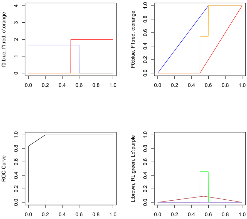
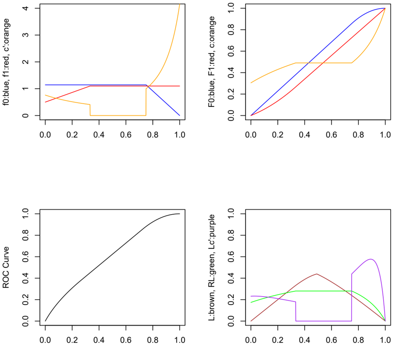
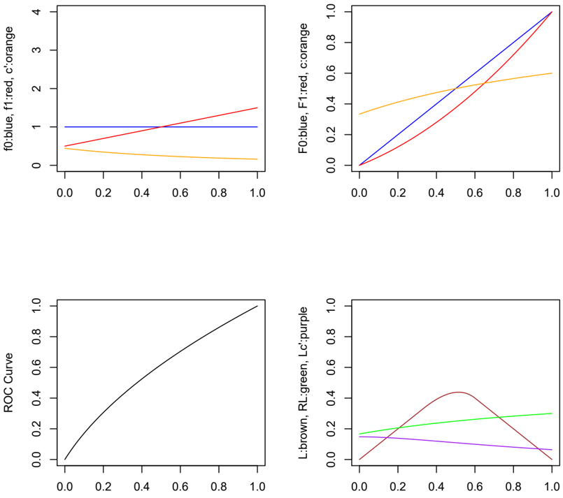
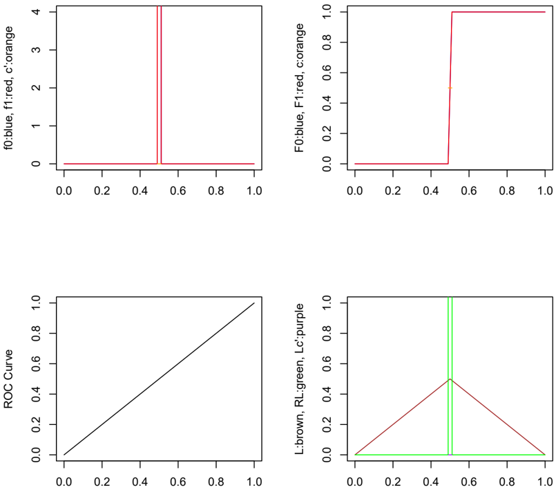
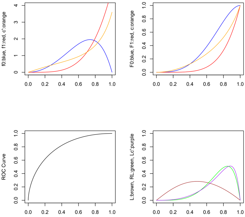
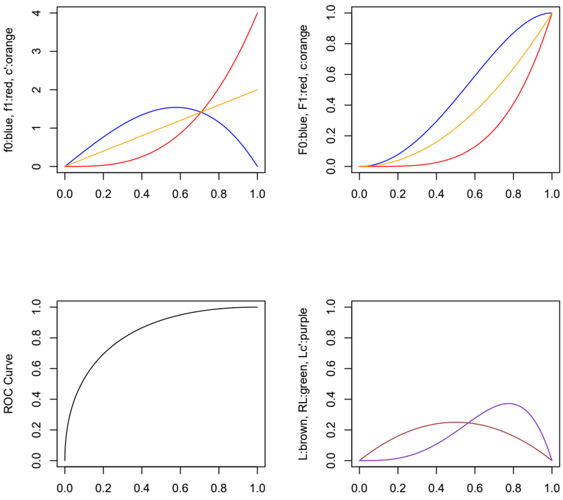
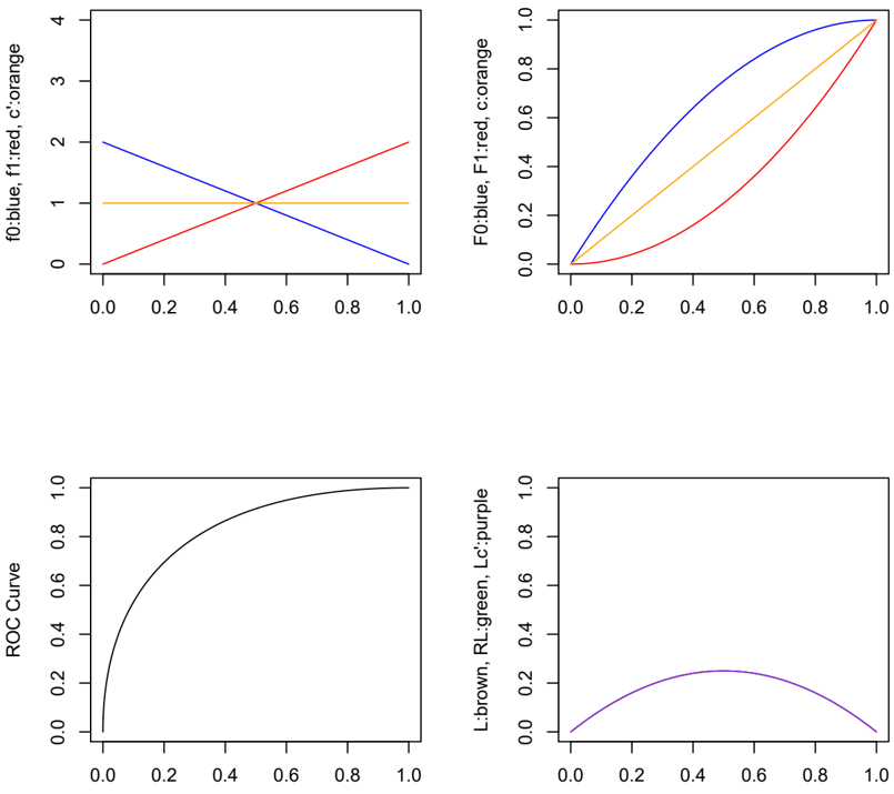
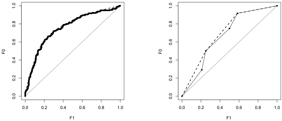
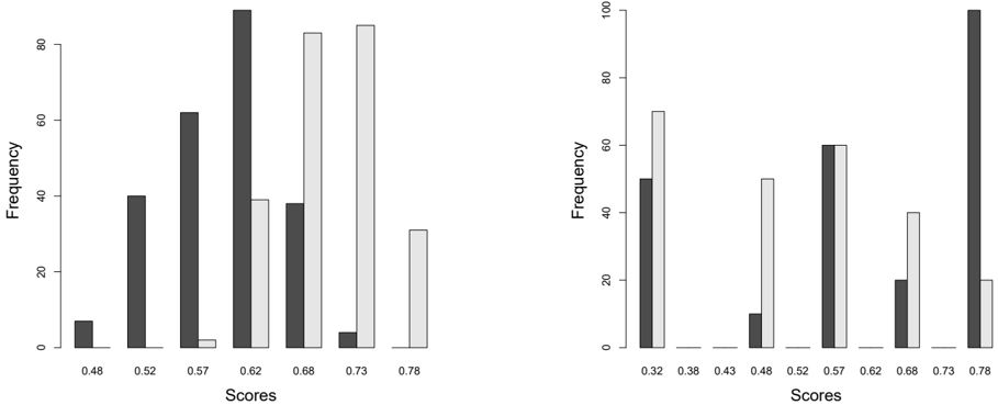
The basic insight is the realisation that there are many ways of converting a model (understood throughout this paper as a function assigning scores to instances) into a classifier that maps instances to classes (we assume binary classification throughout). Put differently, there are many ways of setting the threshold given a model and an operating point. We illustrate this with an example concerning a very common scenario in machine learning research. Consider two models A and B , a naive Bayes model and a decision tree respectively (induced from a training dataset), which are evaluated against a test dataset, producing a score distribution for the positive and negative classes as shown in Figure 1. ROC curves of both models

are shown in Figure 2. We will assume that at this evaluation time we do not have information about the operating condition, but we expect that this information will be available at deployment time .

If we ask the question of which model is best we may rush to calculate its AUC and BS (and perhaps other metrics), as given by Table 1. However, we cannot give an answer because the question is underspecified . First, we need to know the range of operating conditions the model will work with. Second, we need to know how we will make the classifications, or in other words, we need a decision rule , which can be implemented as a threshold choice method when the model outputs scores. For the first dimension (already considered by the work on proper scoring rules), if we have no knowledge about the operating conditions, we can assume a distribution, e.g., a uniform distribution, which considers all operating conditions equally likely. For the second (new) dimension, we have many options.

Table 1: Results from two models on a data set.

performance metric	model A	model B
AUC	0.79	0.67
Brier score	0.33	0.24

For instance, we can just set a fixed threshold at 0.5. This is what naive Bayes and decision trees do by default. This decision rule works as follows: if the score is greater than 0.5 then predict positive, otherwise predict negative. With this precise decision rule, we can now ask the question about the expected loss. Assuming a uniform distribution for operating conditions, we can effectively calculate the answer on the dataset: 0 . 51.

But we can use better decision rules. We can use decision rules which adapt to the operating condition. One of these decision rules is the score-driven threshold choice method, which sets the threshold equal to the operating condition or, more precisely, to a cost proportion c . Another decision rule is the rate-driven threshold choice method, which sets the threshold in such a way that the proportion of predicted positives (or predicted positive rate), simply known as 'rate' and denoted by r , equals the operating condition. Using these three different threshold choice methods for the models A and B we get the expected losses shown in Table 2.

Table 2: Extension of Table 1 where two models are applied with three different threshold choice methods each, leading to six different classifiers and corresponding expected losses. In all cases, the expected loss is calculated over a range of cost proportions (operating conditions), which is assumed to be uniformly distributed. We denote the threshold by T , the cost proportion by c and the predicted positive rate by r ).

threshold choice method	expected loss model A	expected loss model B
Fixed ( T = 0 . 5)	0.510	0.375
Score-driven ( T = c )	0.328	0.231
Rate-driven ( T s.t. r = c )	0.188	0.248

In other words, only when we specify or assume a threshold choice method can we convert a model into a classifier for which it makes sense to consider its expected loss. In fact, as we can see in Table 2, very different expected losses are obtained for the same model with different threshold choice methods. And this is the case even assuming the same uniform cost distribution for all of them.

Once we have made this (new) dimension explicit, we are ready to ask new questions. How many threshold choice methods are there? Table 3 shows six of the threshold choice methods we will analyse in this work, along with their notation. Only the score-fixed and the score-driven methods have been analysed in previous works in the area of proper scoring rules. In addition, a seventh threshold choice method, known as optimal threshold choice method, denoted by T o , has been (implicitly) used in a few works [9, 10, 26].

Table 3: Non-optimal threshold choice methods. The first family uses scores (as they were probabilities) and the second family uses rates (using scores as rank indicators). For both families we can fix a threshold or assume them ranging uniformly, which makes the threshold choice method independent from the operating condition. Only the last column takes the operating condition (o.c.) into account, and hence are the most interesting threshold choice methods.

Threshold choice method	Fixed	Chosen uniformly	Driven by o.c.
Using scores Using rates	score-fixed ( T s f ) rate-fixed ( T r f )	score-uniform ( T su ) rate-uniform ( T ru )	score-driven ( T sd ) rate-driven ( T rd )

We will see that each threshold choice method is linked to a specific performance metric. This means that if we decide (or are forced) to use a threshold choice method then there is a recommended performance metric for it. The results in this paper show that accuracy is the appropriate performance metric for the score-fixed method, MAE fits the score-uniform method, BS is the appropriate performance metric for the score-driven method, and AUC fits both the rate-uniform and the rate-driven methods. All these results assume a uniform cost distribution.

The good news is that inter-comparisons are still possible: given a threshold choice method we can calculate expected loss from the relevant performance metric. The results in Table 2 allow us to conclude that model A achieves the lowest expected loss for uniformly sampled cost proportions, if we are wise enough to choose the appropriate threshold choice method (in this case the rate-driven method) to turn model A into a successful classifier. Notice that this cannot be said by just looking at Table 1 because the metrics in this table are not comparable to each other. In fact, there is no single performance metric that ranks the models in the correct order, because, as already said, expected loss cannot be calculated for models, only for classifiers.

1.1 Contributions and structure of the paper

The contributions of this paper to the subject of model evaluation for classification can be summarised as follows.

1. The expected loss of a model can only be determined if we select a distribution of operating conditions and a threshold choice method. We need to set a point in this two-dimensional space. Along the second (usually neglected) dimension, several new threshold choice methods are introduced in this paper.
2. We answer the question: 'if one is choosing thresholds in a particular way, which performance metric is appropriate?' by giving an explicit expression for the expected loss for each threshold choice method. We derive linear relationships between expected loss and many common performance metrics. The most remarkable one is the vindication of AUC as a measure of expected classification loss for both the rate-uniform and rate-driven methods, contrary to recent claims in the literature [26].

1. One fundamental and novel result shows that the refinement loss of the convex hull of a ROC curve is equal to expected optimal loss as measured by the area under the optimal cost curve. This sets an optimistic (but also unrealistic) bound for the expected loss.
2. Conversely, from the usual calculation of several well-known performance metrics we can derive expected loss. Thus, classifiers and performance metrics become easily comparable. With this we do not choose the best model (a concept that does not make sense) but we choose the best classifier (a model with a particular threshold choice method).
3. By cleverly manipulating scores we can connect several of these performance metrics, either by the notion of evenly-spaced scores or perfectly calibrated scores. This provides an additional way of analysing the relation between performance metrics and, of course, threshold choice methods.
4. We use all these connections to better understand which threshold choice method should be used, and in which cases some are better than others. The analysis of calibration plays a central role in this understanding, and also shows that non-proper scoring rules do have their role and can lead to lower expected loss than proper scoring rules, which are, as expected, more appropriate when the model is well-calibrated.

This set of contributions provides an integrated perspective on performance metrics for classification around the 'missing link' which we develop in this paper: the notion of threshold choice method.

The remainder of the paper is structured as follows. Section 2 introduces some notation, the basic definitions for operating condition, threshold, expected loss, and particularly the notion of threshold choice method, which we will use throughout the paper. Section 3 investigates expected loss for fixed threshold choice methods (score-fixed and rate-fixed), which are the base for the rest. We show that, not surprisingly, the expected loss for these threshold choice method are the 0-1 loss (accuracy or macro-accuracy depending on whether we use cost proportions or skews). Section 4 presents the results that the score-uniform threshold choice method has MAE as associate performance metric and the score-driven threshold choice method leads to the Brier score. We also show that one dominates over the other. Section 5 analyses the non-fixed methods based on rates. Somewhat surprisingly, both the rate-uniform threshold choice method and the ratedriven threshold choice method lead to linear functions of AUC , with the latter always been better than the former. All this vindicates the rate-driven threshold choice method but also AUC as a performance metric for classification. Section 6 uses the optimal threshold choice method, connects the expected loss in this case with the area under the optimal cost curve, and derives its corresponding metric, which is refinement loss, one of the components of the Brier score decomposition. Section 7 analyses the connections between the previous threshold choice methods and metrics by considering several properties of the scores: evenlyspaced scores and perfectly calibrated scores. This also helps to understand which threshold choice method should be used depending on how good scores are. Finally, Section 8 closes the paper with a thorough discussion of results, related work, and an overall conclusion with future work and open questions. There is an appendix which includes some technical results for the optimal threshold choice method and some examples.

2 Background

In this section we introduce some basic notation and definitions we will need throughout the paper. Some other definitions will be delayed and introduced when needed. The most important definitions we will need are introduced below: the notion of threshold choice method and the expression of expected loss.

2.1 Notation and basic definitions

A classifier is a function that maps instances x from an instance space X to classes y from an output space Y . For this paper we will assume binary classifiers, i.e., Y = { 0 , 1 } . A model is a function m : X → R that maps examples to real numbers (scores) on an unspecified scale. We use the convention that higher scores express a stronger belief that the instance is of class 1. A probabilistic model is a function m : X → [ 0 , 1 ] that maps examples to estimates ˆ p ( 1 | x ) of the probability of example x to be of class 1. In order to make predictions in the Y domain, a model can be converted to a classifier by fixing a decision threshold t on the scores. Given a predicted score s = m ( x ) , the instance x is classified in class 1 if s > t , and in class 0 otherwise.

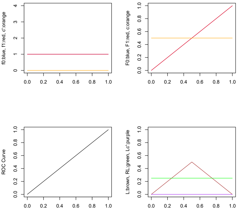
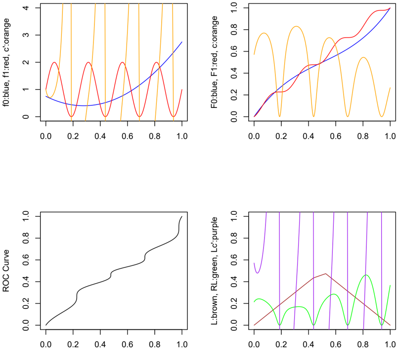
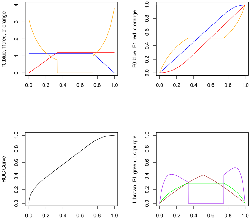
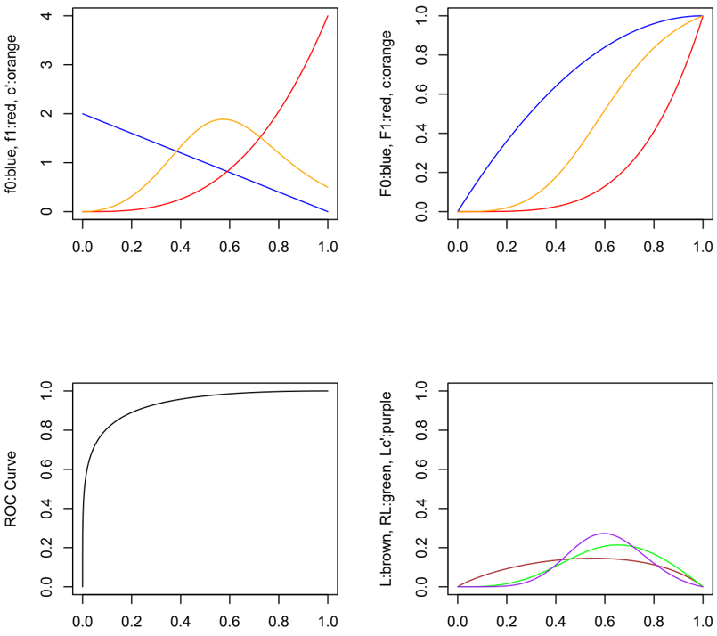
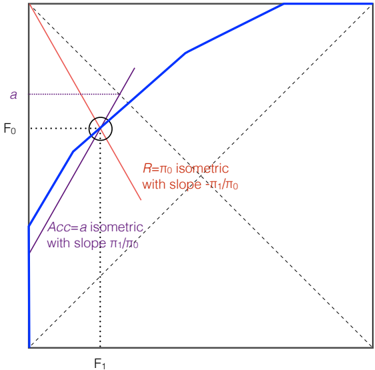
For a given, unspecified model and population from which data are drawn, we denote the score density for class k by f k and the cumulative distribution function by Fk . Thus, F 0 ( t ) = ∫ t -¥ f 0 ( s ) ds = P ( s ≤ t | 0 ) is the proportion of class 0 points correctly classified if the decision threshold is t , which is the sensitivity or true positive rate at t . Similarly, F 1 ( t ) = ∫ t -¥ f 1 ( s ) ds = P ( s ≤ t | 1 ) is the proportion of class 1 points incorrectly classified as 0 or the false positive rate at threshold t ; 1 -F 1 ( t ) is the true negative rate or specificity. Note that we use 0 for the positive class and 1 for the negative class, but scores increase with ˆ p ( 1 | x ) . That is, F 0 ( t ) and F 1 ( t ) are monotonically non-decreasing with t . This has some notational advantages and is the same convention as used by, e.g., Hand [26].

Given a dataset D ⊂〈 X , Y 〉 of size n = | D | , we denote by Dk the subset of examples in class k ∈ { 0 , 1 } , and set nk = | Dk | and p k = nk / n . Clearly p 0 + p 1 = 1. We will use the term class proportion for p 0 (other terms such as 'class ratio' or 'class prior' have been used in the literature). Given a model and a threshold t , we denote by R ( t ) the predicted positive rate, i.e., the proportion of examples that will be predicted positive (class 0) is threshold is set at t . This can also be defined as R ( t ) = p 0 F 0 ( t ) + p 1 F 1 ( t ) . The average score of actual class k is sk = ∫ 1 0 s f k ( s ) ds . Given any strict order for a dataset of n examples we will use the index i on that order to refer to the i -th example. Thus, si denotes the score of the i -th example and yi its true class.

We define partial class accuracies as Acc 0 ( t ) = F 0 ( t ) and Acc 1 ( t ) = 1 -F 1 ( t ) . From here, (microaverage) accuracy is defined as Acc ( t ) = p 0 Acc 0 ( t ) + p 1 Acc 1 ( t ) and macro-average accuracy MAcc ( t ) = ( Acc 0 ( t ) + Acc 1 ( t )) / 2.

We denote by US ( x ) the continuous uniform distribution of variable x over an interval S ⊂ R . If this interval S is [ 0 , 1 ] then S can be omitted. The family of continuous distributions Beta is denoted by B a , b . The Beta distributions are always defined in the interval [ 0 , 1 ] . Note that the continuous distribution is a special case of the Beta family, i.e., B 1 , 1 = U .

2.2 Operating conditions and expected loss

When a model is deployed for classification, the conditions might be different to those during training. In fact, a model can be used in several deployment contexts, with different results. A context can entail different class distributions, different classification-related costs (either for the attributes, for the class or any other kind of cost), or some other details about the effects that the application of a model might entail and the severity of its errors. In practice, a deployment context or operating condition is usually defined by a misclassification cost function and a class distribution. Clearly, there is a difference between operating when the cost of misclassifying 0 into 1 is equal to the cost of misclassifying 1 into 0 and doing so when the former is ten times the latter. Similarly, operating when classes are balanced is different from when there is an overwhelming majority of instances of one class.

One general approach to cost-sensitive learning assumes that the cost does not depend on the example but only on its class. In this way, misclassification costs are usually simplified by means of cost matrices, where we can express that some misclassification costs are higher than others [11]. Typically, the costs of correct classifications are assumed to be 0. This means that for binary models we can describe the cost matrix by two values ck ≥ 0, representing the misclassification cost of an example of class k . Additionally,

we can normalise the costs by setting b = c 0 + c 1 and c = c 0 / b ; we will refer to c as the cost proportion . Since this can also be expressed as c =( 1 + c 1 / c 0 ) -1 , it is often called 'cost ratio' even though, technically, it is a proportion ranging between 0 and 1.

The loss which is produced at a decision threshold t and a cost proportion c is then given by the formula:

This notation assumes the class distribution to be fixed. In order to take both class proportion and cost proportion into account we introduce the notion of skew , which is a normalisation of their product:

From equation (1) we obtain

This gives an expression for loss at a threshold t and a skew z . We will assume that the operating condition is either defined by the cost proportion (using a fixed class distribution) or by the skew. We then have the following simple but useful result.

Proof. If classes are balanced we have c 0 p 0 + c 1 p 1 = b / 2, and the result follows from Equation (2) and Equation (3).

This justifies taking b = 2, which means that Qz and Qc are expressed on the same 0-1 scale, and are also commensurate with error rate which assumes c 0 = c 1 = 1. The upshot of Lemma 1 is that we can transfer any expression for loss in terms of cost proportion to an equivalent expression in terms of skew by just setting p 0 = p 1 = 1 / 2 and z = c . Notice that if c 0 = c 1 = 1 then z = p 0, so in that case skew denotes the class distribution as operating condition.

It is important to distinguish the information we may have available at each stage of the process. At evaluation time we may not have some information that is available later, at deployment time. In many real-world problems, when we have to evaluate or compare models, we do not know the cost proportion or skew that will apply during deployment. One general approach is to evaluate the model on a range of possible operating points. In order to do this, we have to set a weight or distribution on cost proportions or skews. In this paper, we will mostly consider the continuous uniform distribution U (but other distribution families, such as the Beta distribution could be used).

A key issue when applying a model under different operating conditions is how the threshold is chosen in each of them. If we work with a classifier, this question vanishes, since the threshold is already settled. However, in the general case when we work with a model, we have to decide how to establish the threshold. The key idea proposed in this paper is the notion of a threshold choice method, a function which converts an operating condition into an appropriate threshold for the classifier.

Definition 1. Threshold choice method . A threshold choice method is a (possibly non-deterministic) function T : [ 0 , 1 ] → R such that given an operating condition it returns a decision threshold. The operating condition can be either a skew z or a cost proportion c; to differentiate these we use the subscript z or c on T. Superscripts are used to identify particular threshold choice methods. Some threshold choice methods we consider in this paper take additional information into account, such as a default threshold or a target predicted positive rate; such information is indicated by square brackets. So, for example, the score-fixed threshold choice method for cost proportions considered in the next section is indicated thus: T s f c [ t ]( c ) .

When we say that T may be non-deterministic, it means that the result may depend on a random variable and hence may itself be a random variable according to some distribution.

We introduce the threshold choice method as an abstract concept since there are several reasonable options for the function T , essentially because there may be different degrees of information about the model and the operating conditions at evaluation time. We can set a fixed threshold ignoring the operating condition; we can set the threshold by looking at the ROC curve (or its convex hull) and using the cost proportion or the skew to intersect the ROC curve (as ROC analysis does); we can set a threshold looking at the estimated scores, especially when they represent probabilities; or we can set a threshold independently from the rank or the scores. The way in which we set the threshold may dramatically affect performance. But, not less importantly, the performance metric used for evaluation must be in accordance with the threshold choice method.

In the rest of this paper, we explore a range of different methods to choose the threshold (some deterministic and some non-deterministic). We will give proper definitions of all these threshold choice methods in its due section.

Given a threshold choice function Tc , the loss for a particular cost proportion is given by Qc ( Tc ( c ) ; c ) . Following Adams and Hand [1] we define expected loss as a weighted average over operating conditions.

Definition 2. Given a threshold choice method for cost proportions Tc and a probability density function over cost proportions wc, expected loss Lc is defined as

Incorporating the class distribution into the operating condition we obtain expected loss over a distribution of skews:

It is worth noting that if we plot Qc or Qz against c and z , respectively, we obtain cost curves as defined by [9, 10]. Cost curves are also known as risk curves (see, e.g. [43], where the plot can also be shown in terms of priors , i.e., class proportions).

Equations (4) and (5) illustrate the space we explore in this paper. Two parameters determine the expected loss: wc ( c ) and Tc ( c ) (respectively wz ( z ) and Tz ( z ) ). While much work has been done on a first dimension, by changing wc ( c ) or wz ( z ) , particularly in the area of proper scoring rules, no work has systematically analysed what happens when changing the second dimension, Tc ( c ) or Tz ( z ) .

3 Expected loss for fixed-threshold classifiers

The easiest way to choose the threshold is to set it to a pre-defined value t f ixed , independently from the model and also from the operating condition. This is, in fact, what many classifiers do (e.g. Naive Bayes chooses t f ixed = 0 . 5 independently from the model and independently from the operating condition). We will see the straightforward result that this threshold choice method corresponds to 0-1 loss (either micro-average accuracy, Acc , or macro-average accuracy, MAcc ). Part of these results will be useful to better understand some other threshold choice methods.

Definition 3. The score-fixed threshold choice method is defined as follows:

This choice has been criticised in two ways, but is still frequently used. Firstly, choosing 0.5 as a threshold is not generally the best choice even for balanced datasets or for applications where the test distribution is equal to the training distribution (see, e.g. [29] on how to get much more from a Bayes classifier by simply changing the threshold). Secondly, even if we are able to find a better value than 0.5, this does not mean that this value is best for every skew or cost proportion -this is precisely one of the reasons why ROC analysis is used [41]. Only when we know the deployment operating condition at evaluation time is it reasonable to fix the threshold according to this information. So either by common choice or because we have this latter case, consider then that we are going to use the same threshold t independently of skews or cost proportions. Given this threshold choice method, then the question is: if we must evaluate a model before application for a wide range of skews and cost proportions, which performance metric should be used? This is what we answer below.

If we plug T s f c (Equation (6)) into the general formula of the expected loss for a range of cost proportions (Equation (4)) we have:

We obtain the following straightforward result.

Theorem 2. If a classifier sets the decision threshold at a fixed value irrespective of the operating condition or the model, then expected loss under a uniform distribution of cost proportions is equal to the error rate at that decision threshold.

Proof.

In words, the expected loss is equal to the class-weighted average of false positive rate and false negative rate, which is the (micro-average) error rate.

So, the expected loss under a uniform distribution of cost proportions for the score-fixed threshold choice method is the error rate of the classifier at that threshold. That means that accuracy can be seen as a measure of classification performance in a range of costs proportions when we choose a fixed threshold. This interpretation is reasonable, since accuracy is a performance metric which is typically applied to classifiers (where the threshold is fixed) and not to models outputting scores. This is exactly what we did in Table 2. We calculated the expected loss for the fixed threshold at 0.5 for a uniform distribution of cost proportions, and we got 1 -Acc = 0 . 51 and 0 . 375 for models A and B respectively.

Similarly, if we plug T s f z (Equation (6)) into the general formula of the expected loss for a range of skews (Equation (5)) we have:

Using Lemma 1 we obtain the equivalent result for skews:

Corollary 3. If a classifier sets the decision threshold at a fixed value irrespective of the operating condition or the model, then expected loss under a uniform distribution of skews is equal to the macro-average error rate at that decision threshold: L s f U ( z ) ( t ) = ( 1 -F 0 ( t )) / 2 + F 1 ( t ) / 2 = 1 -MAcc ( t ) .

The previous results show that 0-1 losses are appropriate to evaluate models in a range of operating conditions if the threshold is fixed for all of them. In other words, accuracy and macro-accuracy can be the right performance metrics for classifiers even in a cost-sensitive learning scenario. The situation occurs when one assumes a particular operating condition at evaluation time while the classifier has to deal with a range of operating conditions in deployment time.

In order to prepare for later results we also define a particular way of setting a fixed classification threshold, namely to achieve a particular predicted positive rate. One could say that such a method quantifies the proportion of positive predictions made by the classifier. For example, we could say that our threshold is fixed to achieve a rate of 30% positive predictions and the rest negatives. This of course involves ranking the examples by their scores and setting a cutting point at the appropriate position, something which is frequently known as 'screening'.

Definition 4. Define the predicted positive rate at threshold t as R ( t ) = p 0 F 0 ( t ) + p 1 F 1 ( t ) , and assume the cumulative distribution functions F 0 and F 1 are invertible, then we define the rate-fixed threshold choice method for rate r as:

If F 0 and F 1 are not invertible, they have plateaus and so does R. This can be handled by deriving t from the centroid of a plateau.

The rate-fixed threshold choice method for skews is defined as:

where Rz ( t ) = F 0 ( t ) / 2 + F 1 ( t ) / 2 .

The corresponding expected loss for cost proportions is

The notion of setting a threshold based on a rate is closely related to the problem of quantification [21, 4] where the goal is to correctly estimate the proportion for each of the classes (in the binary case, the positive rate is sufficient). This threshold choice method allows the user to set the quantity of positives, which can be known (from a sample of the test) or can be estimated using a quantification method. In fact, some quantification methods can be seen as methods to determine an absolute fixed threshold t that ensures a correct proportion for the test set.

Note that Equation (11) is closely related to Theorem 2. If we determine the threshold which produces a rate, i.e., if we determine R -1 ( r ) , we get the expected loss as an accuracy. Formally, we have:

Fortunately, it is immediate to get the threshold which produces a rate; it can just be derived by sorting the examples by their scores and placing the cutpoint where the rate equals the rank divided by the number of examples (e.g. if we have n examples, the cutpoint i makes r = i / n ).

4 Threshold choice methods using scores

In the previous section we looked at accuracy and error rate as performance metrics for classifiers and gave their interpretation as expected losses. In this and the following sections we consider performance metrics for models that do not require fixing a threshold choice method in advance. Such metrics include AUC

which evaluates ranking performance and the Brier score or mean squared error which evaluates the quality of probability estimates. We will deal with the latter in this section. We will therefore assume that scores range between 0 and 1 and represent posterior probabilities for class 1. This means that we can sample thresholds uniformly or derive them from the operating condition. We first introduce two performance metrics that are applicable to probabilistic scores.

The Brier score is a well-known performance metric for probabilistic models. It is an alternative name for the Mean Squared Error or MSE loss [5], especially for binary classification.

Definition 5. BS ( m , D ) denotes the Brier score of model m on data D; we will usually omit m and D when clear from the context. BS is defined as follows:

From here, we can define a prior-independent version of the Brier score (or a macro-average Brier score) as follows:

The Mean Absolute Error ( MAE ) is another simple performance metric which has been rediscovered many times under different names.

Definition 6. MAE ( m , D ) denotes the Mean Absolute Error of model m on data D; we will again usually omit m and D when clear from the context. MAE is defined as follows:

We can define a macro-average MAE as follows:

It can be shown that MAE is equivalent to the Mean Probability Rate (MPR) [30] for discrete classification [17].

4.1 The score-uniform threshold choice method leads to MAE

We now demonstrate how varying a model's threshold leads to an expected loss that is different from accuracy. First, we explore a threshold choice method which considers that we have no information at all about the operating condition, neither at evaluation time nor at deployment time. We just employ the interval between the maximum and minimum value of the scores, and we randomly select the threshold using a uniform distribution over this interval.

Definition 7. Assuming a model's scores are expressed on a bounded scale [ l , u ] , the score-uniform threshold choice method is defined as follows:

Given this threshold choice method, then the question is: if we must evaluate a model before application for a wide range of skews and cost proportions, which performance metric should be used?

Theorem 4. Assuming probabilistic scores and the score-uniform threshold choice method, expected loss under a uniform distribution of cost proportions is equal to the model's mean absolute error.

Proof. First of all we note that the threshold choice method does not take the operating condition c into account, and hence we can work with c = 1 / 2. Then,

The last step makes use of the following useful property.

Setting l = 0 and u = 1 for probabilistic scores, we obtain the final result:

This gives a baseline loss if we choose thresholds randomly and independently of the model. Using Lemma 1 we obtain the equivalent result for skews:

Corollary 5. Assuming probabilistic scores and the score-uniform threshold choice method, expected loss under a uniform distribution of skews is equal to the model's macro-average mean absolute error:

4.2 The score-driven threshold choice method leads to the Brier score

We will now consider the first threshold choice method to take the operating condition into account. Since we are dealing with probabilistic scores, this method simply sets the threshold equal to the operating condition (cost proportion or skew). This is a natural criterion as it has been used especially when the model is a probability estimator and we expect to have perfect information about the operating condition at deployment time. In fact, this is a direct choice when working with proper scoring rules, since when rules are proper, scores are assumed to be a probabilistic assessment. The use of this threshold choice method can be traced back to Murphy [32] and, perhaps, implicitly, much earlier. More recently, and in a different context from proper scoring rules, Drummond and Holte [10] say it is a common example of a 'performance independence criterion'. Referring to figure 22 in their paper which uses the score-driven threshold choice they say: 'the performance independent criterion, in this case, is to set the threshold to correspond to the operating conditions. For example, if PC (+) = 0 . 2 the Naive Bayes threshold is set to 0.2'. The term PC (+) is equivalent to our 'skew'.

Definition 8. Assuming model's scores are expressed on a probability scale [ 0 , 1 ] , the score-driven threshold choice method is defined for cost proportions as follows:

and for skews as

Given this threshold choice method, then the question is: if we must evaluate a model before application for a wide range of skews and cost proportions, which performance metric should be used? This is what we answer below.

Theorem 6 ([28]) . Assuming probabilistic scores and the score-driven threshold choice method, expected loss under a uniform distribution of cost proportions is equal to the model's Brier score.

Proof. If we plug T sd c (Equation (16)) into the general formula of the expected loss (Equation (4)) we have the expected score-driven loss:

And if we use the uniform distribution and the definition of Qc (Equation (1)):

In order to show this is equal to the Brier score, we expand the definition of BS 0 and BS 1 using integration by parts:

Taking their weighted average, we obtain

which, after reordering of terms and change of variable, is the same expression as Equation (19).

It is now clear why we just put the Brier score from Table 1 as the expected loss in Table 2. We calculated the expected loss for the score-driven threshold choice method for a uniform distribution of cost proportions as its Brier score.

Theorem 6 was obtained in [28] (the threshold choice method there was called 'probabilistic') but it is not completely new in itself. In [32] we find a similar relation to expected utility (in our notation, -( 1 / 4 ) PS +( 1 / 2 )( 1 + p 0 ) , where the so-called probability score PS = 2 BS ). Apart from the sign (which is explained because Murphy works with utilities and we work with costs), the difference in the second constant term is explained because Murphy's utility (cost) model is based on a cost matrix where we have a cost for one of the classes (in meteorology the class 'protect') independently of whether we have a right or wrong prediction ('adverse' or 'good' weather). The only case in the matrix with a 0 cost is when we have 'good' weather and 'no protect'. It is interesting to see that the result only differs by a constant term, which supports the idea that whenever we can express the operating condition with a cost proportion or skew, the results will be portable to each situation with the inclusion of some constant terms (which are the same for all classifiers). In addition to this result, it is also worth mentioning another work by Murphy [33] where he makes a general derivation for the Beta distribution.

After Murphy, in the last four decades, there has been extensive work on the so-called proper scoring rules, where several utility (cost) models have been used and several distributions for the cost have been used. This has led to relating Brier score (square loss), logarithmic loss, 0-1 loss and other losses which take the scores into account. For instance, in [7] we have a comprehensive account of how all these losses can be obtained as special cases of the Beta distribution. The result given in Theorem 6 would be a particular case for the uniform distribution (which is a special case of the Beta distribution) and a variant of Murphy's results. Nonetheless, it is important to remark that the results we have just obtained in Section 4.1 (and those we will get in Section 5) are new because they are not obtained by changing the cost distribution but rather by changing the threshold choice method. The threshold choice method used (the score-driven one) is not put into question in the area of proper scoring rules. But Theorem 6 can now be seen as a result which connects these two different dimensions: cost distribution and threshold choice method, so placing the Brier score at an even more predominant role.

We can derive an equivalent result using empirical distributions [28]. In that paper we show how the loss can be plotted in cost space, leading to the Brier curve whose area below is the Brier score.

Finally, using skews we arrive at the prior-independent version of the Brier score.

It is interesting to analyse the relation between L su U ( c ) and L sd U ( c ) (similarly between L su U ( z ) and L sd U ( z ) ). Since the former gives the MAE and the second gives the Brier score (which is the MSE), from the definitions of MAE and Brier score, we get that, assuming scores are between 0 and 1 we have:

Since MAE and BS have the same terms but the second squares them, and all the values which are squared are between 0 and 1, then the BS must be lower or equal. This is natural, since the expected loss is lower if we get reliable information about the operating condition at deployment time. So, the difference between the Brier score and MAE is precisely the gain we can get by having (and using) the information about the operating condition at deployment time. Notice that all this holds regardless of the quality of the probability estimates.

5 Threshold choice methods using rates

We show in this section that AUC can be translated into expected loss for varying operating conditions in more than one way, depending on the threshold choice method used. We consider two threshold choice methods, where each of them sets the threshold to achieve a particular predicted positive rate: the rateuniform method, which sets the rate in a uniform way; and the rate-driven method, which sets the rate equal to the operating condition.

We recall the definition of a ROC curve and its area first.

Definition 9. The ROC curve [46, 13] is defined as a plot of F 1 ( t ) (i.e., false positive rate at decision threshold t) on the x-axis against F 0 ( t ) (true positive rate at t) on the y-axis, with both quantities monotonically non-decreasing with increasing t (remember that scores increase with ˆ p ( 1 | x ) and 1 stands for the negative class). The Area Under the ROC curve (AUC) is defined as:

5.1 The rate-uniform threshold choice method leads to AUC

The rate-fixed threshold choice method places the threshold in such a way that a given predictive positive rate is achieved. However, if this proportion may change easily or we are not going to have (reliable) information about the operating condition at deployment time, an alternative idea is to consider a nondeterministic choice or a distribution for this quantity. One reasonable choice can be a uniform distribution.

Definition 10. The rate-uniform threshold choice method non-deterministically sets the threshold to achieve a uniformly randomly selected rate:

In other words, it sets a relative quantity (from 0% positives to 100% positives) in a uniform way, and obtains the threshold from this uniform distribution over rates. Note that for a large number of examples, this is the same as defining a uniform distribution over examples or, alternatively, over cutpoints (between examples), as explored in [20].

There are reasons for considering this threshold a reasonable method. It is a generalisation of the ratefixed threshold choice method which considers all the imbalances (class proportions) equally likely whenever we make a classification. It assumes that we will not have any information about the operating condition at deployment time.

As done before for other threshold choice methods, we analyse the question: given this threshold choice method, if we must evaluate a model before application for a wide range of skews and cost proportions, which performance metric should be used?

The corresponding expected loss for cost proportions is

We then have the following result.

Theorem 8 ([20]) . Assuming the rate-fixed threshold choice method, expected loss for uniform cost proportion and uniform rate decreases linearly with AUC as follows:

Proof. First of all we note that the threshold choice method does not take the operating condition c into account, and hence we can work with c = 1 / 2. Furthermore, r = R ( t ) and hence dr = R ′ ( t ) dt = { p 0 f 0 ( t ) + p 1 f 1 ( t ) } dt . Then,

The first term can be related to AUC :

The remaining two terms are easily solved:

Putting everything together we obtain L ru U ( c ) = 2 p 0 p 1 ( 1 -AUC )+( p 2 0 + p 2 1 ) / 2. Since p 0 p 1 +( p 2 0 + p 2 1 ) / 2 = ( p 0 + p 1 ) 2 / 2 = 1 / 2, this can be rewritten to L ru U ( c ) = p 0 p 1 ( 1 -2 AUC ) + 1 / 2. 1

Corollary 9. Assuming the rate-fixed threshold choice method, expected loss for uniform skew and uniform rate decreases linearly with AUC as follows:

We see that expected loss for uniform skew ranges from 1/4 for a perfect ranker that is harmed by suboptimal threshold choices, to 3/4 for the worst possible ranker that puts positives and negatives the wrong way round, yet gains some performance by putting the threshold at or close to one of the extremes.

Intuitively, these formulae can be understood as follows. Setting a randomly sampled rate is equivalent to setting the decision threshold to the score of a randomly sampled example. With probability p 0 we select a positive and with probability p 1 we select a negative. If we select a positive, then the expected true positive rate is 1 / 2 (as on average we select the middle one); and the expected false positive rate is 1 -AUC (as one interpretation of AUC is the expected proportion of negatives ranked correctly wrt. a random positive). Similarly, if we select a negative then the expected true positive rate is AUC and the expected false positive rate is 1 / 2. Put together, the expected true positive rate is p 0 / 2 + p 1 AUC and the expected false positive rate is p 1 / 2 + p 0 ( 1 -AUC ) . The proportion of true positives among all examples is thus

and the proportion of false positives is

We can summarise these expectations in the following contingency table (all numbers are proportions relative to the total number of examples):

	Predicted +	Predicted -
Actual +	p 2 0 / 2 + p 0 p 1 AUC	p 2 0 / 2 + p 0 p 1 ( 1 - AUC )	p 0
Actual -	p 2 1 / 2 + p 0 p 1 ( 1 - AUC )	p 2 1 / 2 + p 0 p 1 AUC	p 1
	1 / 2	1 / 2	1

The column totals are, of course, as expected: if we randomly select an example to split on, then the expected split is in the middle.

While in this paper we concentrate on the case where we have access to population densities f k ( s ) and distribution functions Fk ( t ) , in practice we have to work with empirical estimates. In [20] we provide an alternative formulation of the main results in this section, relating empirical loss to the AUC of the empirical ROC curve. For instance, the expected loss for uniform skew and uniform instance selection is calculated in [20] to be ( n n + 1 ) 1 -2 AUC 4 + 1 2 , showing that for smaller samples the reduction in loss due to AUC is somewhat smaller.

1 If we do not assume a uniform distribution for cost proportions U ( c ) we would obtain a different integral, but expected loss would still be linear in AUC (David Hand, personal communication).

5.2 The rate-driven threshold choice method leads to AUC

Naturally, if we can have precise information of the operating condition at deployment time, we can use the information about the skew or cost to adjust the rate of positives and negatives to that proportion. This leads to a new threshold selection method: if we are given skew (or cost proportion) z (or c ), we choose the threshold t in such a way that we get a proportion of z (or c ) positives. This is an elaboration of the rate-fixed threshold choice method which does take the operating condition into account.

Definition 11. The rate-driven threshold choice method for cost proportions is defined as

The rate-driven threshold choice method for skews is defined as

Given this threshold choice method, the question is again: if we must evaluate a model before application for a wide range of skews and cost proportions, which performance metric should be used? This is what we answer below.

If we plug T rd c (Equation (25)) into the general formula of the expected loss for a range of cost proportions (Equation (4)) we have:

And now, from this definition, if we use the uniform distribution for wc ( c ) , we obtain this new result.

Theorem 10. Expected loss for uniform cost proportions using the rate-driven threshold choice method is linearly related to AUC as follows:

By a change of variable we have c = R ( t ) and hence dc = R ′ ( t ) dt = { p 0 f 0 ( t ) + p 1 f 1 ( t ) } dt = R ′ ( t ) dt , and thus

All terms in the first integral can be reduced to R ( t ) = c :

Proof.

The second integral provides the link to AUC :

And now we can plug this into the expression for the expected loss:

Now we can unveil and understand how we obtained the results for the expected loss in Table 2 for the rate-driven method. We just took the AUC of the models and applied the previous formula: p 1 p 0 ( 1 -2 AUC ) + 1 3 .

Corollary 11. Expected loss for uniform skews using the rate-driven threshold choice method is linearly related to AUC as follows:

If we compare Corollary 9 with Corollary 11, we see that L ru U ( z ) > L rd U ( z ) , more precisely:

So we see that taking the operating condition into account when choosing thresholds based on rates reduces the expected loss with 1 / 6, regardless of the quality of the model as measured by AUC . This term is clearly not negligible and demonstrates that our novel rate-driven threshold choice method is superior to

the rate-uniform method. Figure 3 illustrates this. Logically, L rd U ( c ) and L rd U ( z ) work upon information about the operating condition at deployment time, while L ru U ( c ) and L ru U ( z ) may be suited when this information is unavailable or unreliable.

6 The optimal threshold choice method

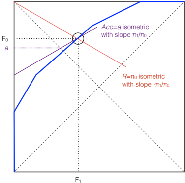
The last threshold choice method we investigate is based on the optimistic assumption that (1) we are having complete information about the operating condition (class proportions and costs) at deployment time and (2) we are able to use that information (also at deployment time) to choose the threshold that will minimise the loss using the current model. ROC analysis is precisely based on these two points since we can calculate the threshold which gives the smallest loss by using the skew and the convex hull.

This threshold choice method, denoted by T o c , is defined as follows:

Definition 12. The optimal threshold choice method is defined as:

and similarly for skews:

A related expression we will also use is:

Note that in both cases, the argmin will typically give a range (interval) of values which give the same optimal value. So these methods can be considered non-deterministic. This threshold choice method is analysed by [15], and used by [9, 10] for defining their cost curves and by [26] to define a new performance metric.

If we plug Equations (28) and (1) into Equation (4) using a uniform distribution for cost proportions, we get:

The connection with the convex hull of a ROC curve (ROCCH) is straightforward. The convex hull is a construction over the ROC curve in such a way that all the points on the convex hull have minimum loss for some choice of c or z . This means that we restrict attention to the optimal threshold for a given cost proportion c , as derived from Equation (28).

6.1 Convexification

We can give a corresponding, and more formal, definition of the convex hull as derived from the score distributions. First, we need a more precise definition of a convex model. For that, we rely on the ROC curve, and we use the slope of the curve, defined as usual:

Sometimes we will use subindices for c ( T ) depending on the model we are using. Clearly, p 0 p 1 slope ( T ) = p 0 f 0 ( T ) p 1 f 1 ( T ) = 1 c ( T ) -1.

Definition 13 (Convex model) . A model m is convex, if for every threshold T, we have that c ( T ) is nondecreasing (or, equivalently, slope ( T ) is non-increasing).

In order to make any model convex, it is not sufficient to repair local concavities, we need to calculate the convex hull. A definition of convex hull for continuous distributions is given as follows:

Definition 14 (Convexification) . Let m be any model with score distributions f 0 ( T ) and f 1 ( T ) . Some values of t will never minimise Qc ( t ; c ) = 2 c p 0 ( 1 -F 0 ( t )) + 2 ( 1 -c ) p 1 F 1 ( t ) } for any value of c. These values will be in one or more intervals of which only the end points will minimise Qc ( t ; c ) for some value of c. We will call these intervals non-hull intervals , and all the rest will be referred to as hull intervals . It clearly holds that hull intervals are convex. Non-hull intervals may contain convex and concave subintervals.

Define convexified score distributions e 0 ( T ) and e 1 ( T ) as follows.

1. For every hull interval ti -1 ≤ s ≤ ti: e 0 ( T ) = f 0 ( T ) and e 1 ( T ) = f 1 ( T ) .
2. For every non-hull interval t j -1 ≤ s ≤ t j :

The function Conv returns the model Conv ( m ) defined by the score distributions e 0 ( T ) and e 1 ( T ) .

We can also define the cumulative distributions Ex ( t ) = ∫ t 0 ex ( T ) dT , where x represents either 0 or 1. By construction we have that for every interval [ t j -1 , t j ] identified above:

and so the convexified score distributions are proper distributions. Furthermore, since the new score distributions are constant in the convexified intervals - and hence monotonically non-decreasing for the new c ( T ) , denoted by c Conv ( m ) ( T ) - so is

It follows that Conv ( m ) is everywhere convex. In addition,

Theorem 12. Optimal loss is invariant under Conv , i.e.: L o U ( c ) ( Conv ( m )) = L o U ( c ) ( m ) for every m.

Proof. By Equation (29) we have that optimal loss is:

By definition, the hull intervals have not been modified by Conv ( m ) . Only the non-hull intervals have been modified. A non-hull interval was defined as those where there is no t which minimises Qc ( t ; c ) = 2 c p 0 ( 1 -F 0 ( t )) + 2 ( 1 -c ) p 1 F 1 ( t ) } for any value of c , and only the endpoints attained the minimum. Consequently, we only need to show that the new e 0 ( T ) and e 1 ( T ) do not introduce any new minima.

We now focus on each non-hull segment ( t j -1 , t j ) using the definition of Conv. We only need to check the expression for the minimum:

From Equation (32) we derive that Ex ( t ) = Ex ( t j -1 ) + ( t j -t j -1 ) ex , j inside the interval (they are straight lines in the ROC curve), and we can see that the expression to be minimised is constant (it does not depend on t ). Since the end points were the old minima and were equal, we see that this expression cannot find new minima.

It is not difficult to see that if we plot Conv ( m ) in the cost space defined by [10] with Qz ( t ; z ) on the y -axis against skew z on the x -axis, we have a cost curve. Its area is then the expected loss for the optimal threshold choice method. In other words, this is the area under the (optimal) cost curve. Similarly, the new performance metric introduced by Hand ( H ) [26] is simply a normalised version of the area under the optimal cost curve using the B 2 , 2 distribution instead of the B 1 , 1 (i.e., uniform) distribution, and using cost proportions instead of skews (so being dependent to class priors). This is further discussed in [20].

6.2 The optimal threshold choice method leads to refinement loss

Once again, the question now must be stated clearly. Assume that the optimal threshold choice method is set as the method we will use for every application of our model. Furthermore, assume that each and every application of the model is going to find the perfect threshold. Then, if we must evaluate a model before application for a wide range of skews and cost proportions, which performance metric should be used? In what follows, we will find the answer by relating this expected loss with a genuine performance metric: refinement loss. We will now introduce this performance metric.

The Brier score, being a sum of squared residuals, can be decomposed in various ways. The most common decomposition of the Brier score is due to Murphy [34] and decomposes the Brier score into Reliability, Resolution and Uncertainty. Frequently, the two latter components are joined together and the decomposition gives two terms: calibration loss and refinement loss.

This decomposition is usually applied to empirical distributions, requiring a binning of the scores. That is, the decomposition is based on a partition P D = { bj } j = 1 .. B where D is the dataset, B the number of bins, and each bin is denoted by bj ⊂ D . Since it is a partition ⋃ B j = 1 bj = D . With this partition the decompoistion is:

Here we use the notation sbj = 1 | bj | GLYPH<229> i ∈ bj si and ybj = 1 | bj | GLYPH<229> i ∈ bj yi for the average predicted scores and the average actual classes respectively for bin bj .

For many partitions the empirical decomposition is not exact. It is only exact for partitions which are coarser than the partition induced by the ROC curve (i.e., ties cannot be spread over different partitions), as shown by [18]. We denote by CL ROC and RL ROC the calibration loss and the refinement loss, respectively, using the segments of the empirical ROC curve as bins. In this case, BS = CL ROC + RL ROC .

In this paper we will use a variant of the above decomposition based on the ROC convex hull of a model. In this decomposition, we take each bin as each segment in the convex hull. Naturally, the number of bins in this decomposition is lower or equal than the number of bins in the ROC decomposition. In fact, we may find different values of si in the same bin. In some way, we can think about this decomposition as an optimistic/optimal version of the ROC decomposition, as Theorem 3 in [18] shows. We denote by CL ROCCH and RL ROCCH the calibration loss and the refinement loss, respectively, using the segments of the convex hull of the empirical ROC curve as bins [20].

We can define the same decomposition in continuous terms considering Definition 5. We can see that in the continuous case, the partition is irrelevant. Any partition will give the same result, since the composition of consecutive integrals is the same as the whole integral.

Theorem 13. The continuous decomposition of the Brier Score, BS = CL + RL, is exact and gives CL and RL as follows.

Proof.

This proof keeps the integral from start to end. That means that the decomposition is not only true for the integral as a whole, but also pointwise for every single score s . Note that ybj in the empirical case (see Definition 33) corresponds to c ( s ) = p 1 f 1 ( s ) p 0 f 0 ( s )+ p 1 f 1 ( s ) (as given by Equation (31)) in the continuous case above, and also note that sbj corresponds to the cardinality p 0 f 0 ( s ) + p 1 f 1 ( s ) . The decomposition for empirical distributions as introduced by [34] is still predominant for any reference to the decomposition. To our knowledge this is the first explicit derivation of a continuous version of the decomposition.

And now we are ready for relating the optimal threshold choice method with a performance metric as follows:

Theorem 14. For every convex model m, we have that:

The proof of this theorem is found in the appendix as Theorem 27. This proof is accompanied with several examples that show that the above correspondence is not pointwise in general. This means that the RL is a genuinely different way of calculating L o U ( c ) ( m ) . In fact, in the appendix, we see that there is a third way of calculating L o U ( c ) ( m ) .

Corollary 15. For every model m the expected loss for the optimal threshold choice method L o U ( c ) is equal to the refinement loss using the convex hull.

It is possible to obtain a version of this theorem for empirical distributions which states that L o U ( c ) = RL ROCCH where RL ROCCH is the refinement loss of the empirical distribution using the segments of the convex hull for the decomposition.

Before better analysing what the meaning of this threshold choice method is and how it relates to the rest, we first have to consider whether this threshold choice method is realistic or not. In the beginning of this section we said that the optimal method assumes that (1) we are having complete information about the operating condition at deployment time and (2) we are able to use that information to choose the threshold that will minimise the loss at deployment time.

While (1) is not always true, there are many occasions where we know the costs and distributions at application time. This is the base of the score-driven and rate-driven methods. However, having this information does not mean that the optimal threshold for a dataset (e.g. the training or validation dataset) ensures an optimal choice for a test set (2). Drummond and Holte [10] are conscious of this problem and they reluctantly rely on a threshold choice method which is based on 'the ROC convex hull [...] only if this selection criterion happens to make cost-minimizing selections, which in general it will not do'. But even if these cost-minimising selections are done, as mentioned above, it is not clear how reliable they are for a test dataset. As Drummond and Holte [10] page 122, recognise: 'there are few examples of the practical application of this technique. One example is [15], in which the decision threshold parameter was tuned to be optimal, empirically, for the test distribution'.

In the example shown in Table 2 in Section 1, the evaluation technique was training and test. However, with cross-validation, the convex hull cannot be estimated reliably in general, and the thresholds derived from each fold might be inconsistent. Even with a big validation dataset, the decision threshold may be suboptimal. This is one of the reasons why the area under the convex hull has not been used as a performance metric. In any case, we can calculate the values as an optimistic limit, leading to L o U ( c ) = RL ROCCH = 0 . 0953 for model A and 0 . 2094 for model B .

7 Relating performance metrics

So far, we have repeatedly answered the following question: 'If threshold choice method X is used, which is the corresponding performance metric?' The answers are summarised in Table 4. The seven threshold choice methods are shown in the first column (the two fixed methods are grouped in the same row). The integrated view of performance metrics for classification is given by the next two columns. The expected loss of a model for a uniform distribution of cost proportions or skews for each of these seven threshold choice methods produces most of the common performance metrics in classification: 0-1 loss (either macroaccuracy or micro-accuracy), the Mean Absolute Error (equivalent to Mean Probability Rate), the Brier score, AUC (which equals the Wilcoxon-Mann-Whitney statistic and the Kendall tau distance of the model to the perfect model, and is linearly related to the Gini coefficient) and, finally, the refinement loss using the bins given by the convex hull.

All the threshold choice methods seen in this paper consider model scores in different ways. Some of them disregard the score, since the threshold is fixed, some others consider the 'magnitude' of the score as an (accurate) estimated probability, leading to the score-based methods, and others consider the 'rank', 'rate' or 'proportion' given by the scores, leading to the rate-based methods. Since the optimal threshold choice is also based on the convex hull, it is apparently more related to the rate-based methods. This is consistent with the taxonomy proposed in [17] based on correlations over more than a dozen performance metrics, where three families of metrics were recognised: performance metrics which account for the quality of

Table 4: Threshold choice methods and their expected loss for cost proportions and skews. The M in MAcc , MMAE , MBS and MRL mean that these metrics are 'macro-averaged', i.e., calculated as if p 0 = p 1.

Threshold choice method	Cost proportions	Skews	Equivalent (or related) performance metrics
fixed	L s f U ( c ) = 1 - Acc	L s f U ( z ) = 1 - MAcc	0-1 loss: Accuracy and macro-accuracy.
score- uniform	L su U ( c ) = MAE	L su U ( z ) = MMAE	Absolute error, Average score, pAUC [16] , Prob- ability Rate [17].
score- driven	L sd U ( c ) = BS	L sd U ( z ) = MBS	Brier score [5], Mean Squared Error ( MSE ).
rate- uniform	L ru U ( c ) = p 0 p 1 ( 1 - 2 AUC )+ 1 2	L ru U ( z ) = 1 - 2 AUC 4 + 1 2	AUC [46] and variants ( m AUC ) [12, 17], Kendall tau, WMWstatistic, Gini coefficient.
rate-driven	L rd U ( c ) = p 0 p 1 ( 1 - 2 AUC )+ 1 3	L rd U ( z ) = 1 - 2 AUC 4 + 1 3	AUC [46] and variants ( m AUC ) [12, 17], Kendall tau, WMWstatistic, Gini coefficient.
optimal	L o U ( c ) = RL Conv	L o U ( z ) = MRL Conv	ROCCH Refinement loss [18], Refinement Loss [34], Area under the Cost Curve ('Total Expected Cost') [10], Hand's H [26].

classification (such as accuracy), performance metrics which account for a ranking quality (such as AUC ), and performance metrics which evaluate the quality of scores or how well the model does in terms of probability estimation (such as the Brier score or logloss).

This suggests that the way scores are distributed is crucial in understanding the differences and connections between these metrics. In addition, this may shed light on which threshold choice method is best. We have already seen some relations, such as L su U ( c ) ≥ L sd U ( c ) , and L ru U ( c ) > L rd U ( c ) , but what about L sd U ( c ) and L rd U ( c ) ? Are they comparable? And what about L o U ( c ) ? It gives the minimum expected loss by definition over the training (or validation) dataset, but when does it become a good estimation of the expected loss for the test dataset?

In order to answer these questions we need to analyse transformations on the scores and see how these affect the expected loss given by each threshold choice method. Given a model, its scores establish a total order over the examples: s =( s 1 , s 2 , ..., sn ) where si ≤ si + 1. Since there might be ties in the scores, this total order is not necessarily strict. A monotonic transformation is any alteration of the scores, such that the order is kept. We will consider two transformations: the evenly-spaced transformation and PAV calibration.

7.1 Evenly-spaced scores. Relating Brier score, MAE and AUC

If we are given a ranking or order, or we are given a set of scores but its reliability is low, a quite simple way to assign (or re-assign) the scores is to set them evenly-spaced (in the [ 0 , 1 ] interval).

Definition 15. A discrete evenly-spaced transformation is a procedure EST ( s ) → s ′ which converts any sequence of scores s =( s 1 , s 2 , ..., sn ) where si < si + 1 into scores s ′ =( s ′ 1 , s ′ 2 , ..., s ′ n ) where s ′ i = i -1 n -1 .

Notice that such a transformation does not affect the ranking and hence does not alter the AUC .

The previous definition can be applied to continuous score distribution as follows:

Definition 16. A continuous evenly-spaced transformation is a any strictly monotonic transformation function on the score distribution, denoted by Even , such that for the new scores s ′ it holds that P ( s ′ ≤ t ) = t.

It is easy to see that EST is idempotent, i.e., EST ( EST ( s )) = EST ( s ) . So we say a set of scores s is evenly-spaced if EST ( s ) = s .

Lemma 16. Given a model and dataset with set of scores s , such that they evenly-spaced, when n → ¥ then we have R ( t ) = t.

Proof. Remember that by definition the true positive rate F 0 ( t ) = P ( s ≤ t | 0 ) and the false positive rate F 1 ( t ) = P ( s ≤ t | 1 ) . Consequently, from the definition of rate we have R ( t ) = p 0 F 0 ( t ) + p 1 F 1 ( t ) = p 0 P ( s ≤ t | 0 ) + p 1 P ( s ≤ t | 1 ) = P ( s ≤ t ) . But, since the scores are evenly-spaced, the number of scores such that s ≤ t is GLYPH<229> n i = 1 I ( si ≤ t ) = GLYPH<229> n i = 1 I ( i -1 n -1 ≤ t ) with I being the indicator function (1 when true, 0 otherwise). This number of scores is GLYPH<229> tn i = 1 1 when n → ¥ , which clearly gives tn . So the probability P ( s ≤ t ) is tn / n = t . Consequently R ( t ) = t .

The following results connect the score-driven threshold choice method with the rate-driven threshold choice method:

Theorem 17. Given a model and dataset with set of scores s , such that they are evenly-spaced, when n → ¥ :

Proof. By Lemma 16 we have R ( t ) = t , and so the rate-driven and score-driven threshold choice methods select the same thresholds.

Corollary 18. Given a model and dataset with set of scores s such that they are evenly-spaced, when n → ¥ :

These straightforward results connect AUC and Brier score for evenly-spaced scores. This connection is enlightening because it says that AUC and BS are equivalent performance metrics (linearly related) when we set the scores in an evenly-spaced way. In other words, it says that AUC is like a Brier score which considers all the scores evenly-spaced. Although the condition is strong, this is the first linear connection which, to our knowledge, has been established so far between AUC and the Brier score.

Similarly, we get the same results for the score-uniform threshold choice method and the rate-uniform threshold choice method.

Theorem 19. Given a model and dataset with set of scores s such that they are evenly-spaced, when n → ¥ :

with similar results for skews. This also connects MAE with AUC and clarifies when they are linearly related.

7.2 Perfectly-calibrated scores. Relating BS , CL and RL

In this section we will work with a different condition on the scores. We will study what interesting connections can be established if we assume the scores to be perfectly calibrated.

The informal definition of perfect calibration usually says that a model is calibrated when the estimated probabilities are close to the true probabilities. From this informal definition, we would derive that a model is perfectly calibrated if the estimated probability given by the scores (i.e., ˆ p ( 1 | x ) ) equals the true probability. However, if this definition is applied to single instances, it implies not only perfect calibration but a perfect model. In order to give a more meaningful definition, the notion of calibration is then usually defined in terms of groups or bins of examples, as we did, for instance, with the Brier score decomposition. So, we need to apply this correspondence between estimated and true (actual) probabilities over bins. We say a bin partition is invariant on the scores if for any two examples with the same score they are in the same bin. In other words, two equal scores cannot be in different bins (equivalence classes cannot be broken). From here,

Definition 17 (Perfectly-calibrated for empirical distribution models) . We say that a model is perfectly calibrated if for any invariant bin partition P we have that ybj = sbj for all its bins: i.e., the average actual probability equals the average estimated probability, thus making CL P = 0 . Note that it is not sufficient to have CL = 0 for one partition, but for all the invariant partitions.

Notice that the bins which are generated by a ROC curve are the minimal invariant partition on the scores (i.e., the quotient set). So, we can give an alternative definition of perfectly calibrated model: a model is perfectly calibrated if and only if CL ROC = 0. For the continuous case, the partition is irrelevant and the definition is as follows:

Definition 18 (Perfectly-calibrated for continuous distribution models) . We say a continuous model is perfectly calibrated if CL = 0 .

Lemma 20. For a perfectly calibrated classifier m:

and c ( s ) = s as defined in Equation (31), which means that m is convex.

Proof. Consider the decomposition of Theorem 13. A perfectly calibrated classifier must have CL = 0 for every single continuous interval. That means that:

which means s = p 1 f 1 ( s ) p 0 f 0 ( s )+ p 1 f 1 ( s ) which is exactly c ( s ) given by Equation (31) and the result and convexity follow (by definition 13).

Now that we have two proper and operational definitions of perfect calibration, we define a calibration transformation as follows.

Definition 19. Cal is a monotonic function over the scores which converts any model m into another calibrated model m ∗ such that CL = 0 and RL is not modified.

glyph[negationslash]

Cal always produces a convex model, so Conv ( Cal ( m )) = Cal ( m ) , but a convex model is not always perfectly calibrated (e.g., a binormal model with same variances is always convex but it can be uncalibrated), so Cal ( Conv ( m ) = Conv ( m ) . This is summarised in Table 5. If the model is strictly convex, then Cal is strictly monotonic. An instance of the function Cal is the transformation T ↦→ s = c ( T ) where c ( T ) = p 1 f 1 ( T ) p 0 f 0 ( T )+ p 1 f 1 ( T ) as given by Equation (31). This transformation is shown to keep RL unchanged in the appendix and makes CL = 0.

The previous function is defined for continuous score distributions. The corresponding function for empirical distributions is known as the Pool Adjacent Algorithm (PA V) [2]. Following [14], the PAV function converts any model m into another calibrated model m ∗ such that the following property sbj = ybj holds for every segment in its convex hull.

It has been shown by [14] that isotonic-based calibration [44] is equivalent to the PA V algorithm, and closely related to ROCCH, since, for every m and dataset, we have:

Table 5: Transformations on scores. Perfect calibration implies a convex model but not vice versa.

	Evenly-spaced	Convexification	Perfect Calibration
Continuous distributions	Even	Conv	Cal
Empirical distributions	EST	ROCCH	PAV

It is also insightful to see that isotonic regression (calibration) is the monotonic function defined as argmin f GLYPH<229> ( yi -f ( si )) 2 , i.e., the monotonic function over the scores which minimises the Brier score. This leads to the same function if we use any other proper scoring function (such as logloss).

The similar expression for the continuous case is

Nowweanalyse what happens with perfectly calibrated models for the score-driven threshold choice and the score-uniform threshold choice methods. This will help us understand the similarities and differences between the threshold choices and their relation with the optimal method. Along the way, we will obtain some straightforward, but interesting, results. We start with a basic result:

Theorem 21. If a model is perfectly calibrated then we have:

Proof. For perfectly calibrated models, we have that for every bin in an invariant partition on the scores we have that ybj = sbj . Just taking a partition consisting of one single bin (which is an invariant partition), we have that this is the same as saying that p 1 = p 1 ¯ s 1 + p 0 ¯ s 0. This leads to p 1 ( 1 -¯ s 1 ) = p 0 ¯ s 0.

This is an interesting equation in its own right. It gives a necessary condition for calibration: the extent to which the average score over all examples (which is the weighted mean of per-class averages p 0 s 0 + p 1 s 1) deviates from p 1.

We now give a first result which connects two performance metrics:

Theorem 22. If a model is perfectly calibrated then we have:

Proof. We use the continuous decomposition (Theorem 13):

Since it is perfectly calibrated, CL = 0. Then we have:

or equivalently,

Since it is perfectly calibrated, we have:

So:

We will now use the expressions for expected loss to analyse where this result comes from exactly. In the following result, we see that for a calibrated model the optimal threshold T for a given cost proportion c is T = c , which is exactly the score-driven threshold choice method. In other words:

Theorem 23. For a perfectly calibrated model: ∀ c : T o c ( c ) = T sd c ( c ) = c

Proof. By Lemma 20 we have

Setting the two slopes equal implies T = c .

And now we can express and relate many of the expressions for the expected loss seen so far. Starting with the expected loss for the optimal threshold choice method, i.e., L o c (which uses T o c ), we have, from Theorem 23, that T o c ( c ) = T sd c ( c ) = c when the model is perfectly calibrated. Consequently, we have the same as Equation (18), and since we know that BS = p 0 ¯ s 0 for perfectly calibrated models, we have:

The following theorem summarises all the previous results.

Theorem 24. For perfectly calibrated models:

Proof. Since L sd U ( c ) = BS it is clear that L sd U ( c ) = p 0 ¯ s 0, as seen above for L o U ( c ) as well. Additionally, from Theorem 4, we have that L su U ( c ) = p 0 s 0 + p 1 ( 1 -s 1 ) , which reduces to 2 L su U ( c ) = 2 BS = 2 p 0 s 0. We also use the result of Theorem 14 which states that, in general (not just for perfectly calibrated models), L o U ( c ) ( m ) = RL ( Conv ( m )) .

All this gives an interpretation of the optimal threshold choice method as a method which calculates expected loss by assuming perfect calibration. Note that this is clearly seen by the relation L sd U ( c ) = L o U ( c ) = L su U ( c ) 2 , since the loss drops to the half if we use scores to adjust to the operating condition. In this situation, we get the best possible result.

If we know c , we want to find the score s = T where the slope is equal to the slope of a cost isometric [19]. The slope of a cost isometric is

General relations: L ru U ( c ) = p 0 p 1 ( 1 -2 AUC ) + 1 2 > L rd U ( c ) = p 0 p 1 ( 1 -2 AUC ) + 1 3 ≥ L o U ( c ) = RL Conv L su U ( c ) = MAE ≥ L sd U ( c ) = BS ≥ L o U ( c ) = RL Conv If scores are evenly-spaced: L ru U ( c ) = p 0 p 1 ( 1 -2 AUC ) + 1 2 = L su U ( c ) = MAE = p 0 ¯ s 0 + p 1 ( 1 -s 1 ) L rd U ( c ) = p 0 p 1 ( 1 -2 AUC ) + 1 3 = L sd U ( c ) = BS If scores are perfectly calibrated: L sd U ( c ) = L o U ( c ) = RL = L su U ( c ) 2 = MAE 2 = BS = p 0 ¯ s 0 = p 1 ( 1 -s 1 ) If the model has perfect ranking: L ru U ( c ) = 1 4 > L rd U ( c ) = 1 12 > L o U ( c ) = 0 If the model is random (and p 0 = p 1): L su U ( c ) = L sd U ( c ) = L ru U ( c ) = 1 2 > L rd U ( c ) = 1 3 > L o U ( c ) = 1 4

Figure 4: Comparison of losses and performance metrics, in general and under several score conditions.

7.3 Choosing a threshold choice method

It is enlightening to see that many of the most popular classification performance metrics are just expected losses by changing the threshold choice method and the use of cost proportions or skews. However, it is even more revealing to see how (and under which conditions) these performance metrics can be related (in some cases with inequalities and in some other cases with equalities). The notion of score transformation is the key idea for these connections, and is more important that it might seem at first sight. Some threshold choice methods can be seen as a score transformation followed by the score-driven threshold choice method. Even the fixed threshold choice method can be seen as a crisp transformation where scores are set to 1 if si > t and 0 otherwise. Another interesting point of view is to see the values of extreme models, such as a model with perfect ranking ( AUC = 1, RL ROCCH = 0) and a random model ( AUC = 0 . 5, RL ROCCH = 0 . 25 when p 0 = p 1). Figure 4 summarises all the relations found so far and these extreme cases.

The first apparent observation is that L o U ( c ) seems the best loss, since it derives from the optimal threshold choice method. We already argued in Section 6 that this is unrealistic. The result given by Theorem 14 is a clear indication of this, since this makes expected loss equal to RL Conv. Hence, this threshold choice method assumes that the calibration which is performed with the convex hull over the training (or a validation dataset) is going to be perfect and hold for the test set. Figure 4 also gives the impression that L su U ( c ) and L ru U ( c ) are so bad that their corresponding threshold choice methods and metrics are useless. In order to refute this simplistic view, we must realise (again) that not every threshold choice method can be applied in every situation. Some require more information or more assumptions than others. Table 6 completes Table 3 to illustrate the point. If we know the deployment operating condition at evaluation time, then we can fix the

threshold and get the expected loss. If we do not know this information at evaluation time, but we expect to be able to have it and use it at deployment time, then the score-driven, rate-driven and optimal threshold choice methods seem the appropriate ones. Finally, if no information about the operating condition is going to be available at any time then the score-uniform and the rate-uniform are the (only reasonable) option.

Table 6: Information which is required (and when) for the seven threshold choice methods so that they become reasonable. Operating condition is denoted by o.c.

Threshold choice method	Fixed	Driven by o.c.	Chosen uniformly
Using scores Using rates Using optimal	score-fixed ( T s f ) rate-fixed ( T r f )	score-driven ( T sd ) rate-driven ( T rd ) optimal ( T o )	score-uniform ( T su ) rate-uniform ( T ru )
Required information	o.c. at evaluation time	o.c. at deployment time	no information
thresholds

From the cases shown in 6, the methods driven by the operating condition require further discussion. The relations shown in Figure 4 illustrate that, in addition to the optimal threshold choice method, the other two methods that seem more competitive are the score-driven and the rate-driven. One can argue that the rate-driven threshold choice has an expected loss which is always greater than 1 / 12 (if AUC = 1, we get -1 / 4 + 1 / 3), while the others can be 0. But things are not so clear-cut.

• The score-driven threshold choice method considers that the scores are estimated probabilities and that they are reliable, in the tradition of proper scoring rules. So it just uses these probabilities to set the thresholds.
• The rate-driven threshold choice method completely ignores the scores and only considers their order. It assumes that the ranking is reliable while the scores are not accurate probabilities. It derives the thresholds using the predictive positive rate. It can be seen as the score-driven threshold choice method where the scores have been set evenly-spaced by a transformation.
• The optimal threshold choice method also ignores the scores completely and only considers their order. It assumes that the ranking is reliable while the scores are not accurate probabilities. However, this method derives the thresholds by keeping the order and using the slopes of the segments of the convex hull (typically constructed over the training dataset or a validation dataset). It can be seen as the score-driven threshold choice method where the scores have been calibrated by the PAV method.

Now that we better understand the meaning of the threshold choice methods we may state the difficult question more clearly: given a model, which threshold choice method should we use to make classifications? The answer is closely related to the calibration problem. Some theoretical and experimental results [44, 2, 39, 47, 48, 37, 36, 3, 22] have shown that the PAV method (also known as isotonic regression) is not frequently the best calibration method. Some other calibration methods could do better, such as Platt's calibration or binning averaging. In particular, it has been shown that 'isotonic regression is more prone to overfitting, and thus performs worse than Platt scaling, when data is scarce' [36]. Even with a large validation dataset which allows the construction of an accurate ROC curve and an accurate convex hull, the resulting choices are not necessarily optimal for the test set, since there might be problems with outliers [45]. In fact, if the validation dataset is much smaller (or biased) than the training set, the resulting probabilities can be even worse than the original probabilities, as it may happen with cross-validation. So, we have to feel free to use other (possibly better) calibration methods instead and do not stick to the PA V method just because it is linked to the optimal threshold choice method.

So the question of whether we keep the scores or not (and how we replace them in case) depends on our expectations on how well-calibrated the model is, and whether we have tools (calibration methods and validation datasets) to calibrate the scores.

But we can turn the previous question into a much more intelligent procedure. Calculating the three expected losses discussed above (and perhaps the other threshold choice methods as well) provides a rich source of information about how our models behave. This is what performance metrics are all about. It is only after the comparison of all the results and the availability of (validation) datasets when we can make a decision about which threshold choice method to use.

This is what we did with the example shown in Table 2 in Section 1. We evaluated the model for several threshold choice methods and from there we clearly saw which models were better calibrated and we finally made a decision about which model to use and with which threshold choice methods.

In any case, note that the results and comparisons shown in Figure 4 are for expected loss; the actual loss does not necessarily follow these inequalities. In fact, the expected loss calculated over a validation dataset may not hold over the test dataset, and even some threshold choice methods we have discarded from the discussion above (the fixed ones or the score-uniform and rate-uniform, if probabilities or rankings are very bad respectively) could be better in some particular situations.

8 Discussion

This paper builds upon the notion of threshold choice method and the expected loss we can obtain for a range of cost proportions (or skews) for each of the threshold choice methods we have investigated. The links between threshold choice methods, between performance metrics, in general and for specific score arrangements, have provided us with a much broader (and more elaborate) view of classification performance metrics and the way thresholds can be chosen. In this last section we link our results to the extensive bulk of work on classification evaluation and analyse the most important contributions and open questions which are derived from this paper.

8.1 Related work

One decade ago there was a scattered view of classification evaluation. Many performance metrics existed and it was not clear what their relationships were. One first step in understanding some of these performance metrics in terms of costs was the notion of cost isometrics [19]. With cost isometrics, many classification metrics (and decision tree splitting criteria) are characterised by its skew landscape, i.e., the slope of its isometric at any point in the ROC space. Another comprehensive view was the empirical evaluation made in [17]. The analysis of Pearson and Spearman correlations between 18 different performance metrics shows the pairs of metrics for which the differences are significant.

In addition to these, there have been three lines of research in this area which provide further pieces to understand the whole picture.

• First, the notion of 'proper scoring rules' (which was introduced in the sixties, see e.g. [35]), has been developed to a degree [7] in which it has been shown that the Brier score (MSE loss), logloss, boosting loss and error rate (0-1 loss) are all special cases of an integral over a Beta density, and that all these performance metrics can be understood as averages (or integrals), at least theoretically, over a range of cost proportions (see e.g. [23, 42, 6]), so generalising the early works by Murphy on probabilistic predictions when cost-loss ratio is unknown ([32] and [33]). Additionally, further connections have been found between proper scoring rules and distribution divergences ( f -divergences and Bregman divergences) [43].

• Second, the translation of the Brier decomposition using ROC curves [18] suggests a connection between the Brier score and ROC curves, and most specially between refinement loss and AUC , since both are performance metrics which do not require the magnitude of the scores of the model.
• Third, an important coup d'effet has been given by Hand [26], stating that the AUC cannot be used as a performance metric for evaluating models (for a range of cost proportions) because the distribution for these cost proportions depends on the model. This seemed to suggest a definitive rupture between ranking quality and classification performance over a range of cost proportions.

Each of the three lines mentioned above provides a partial view of the problem of classifier evaluation, and suggests that some important connections between performance metrics were waiting to be unveiled. The starting point of this unifying view is that all the previous works above worked with only two threshold choice methods, which we have called the score-driven threshold choice method and the optimal threshold choice method. Only a few works mention these two threshold choice methods together. For instance, Drummond and Holte [10] talk about 'selection criteria' (instead of 'threshold choice methods') and they distinguish between 'performance-independent' selection criteria and 'cost-minimizing' selection criteria. Hand (personal communication) says that '[26] (top of page 122) points out that there are situations where one might choose thresholds independently of cost, and go into more detail in [27]'. This is related to the fixed threshold choice method, or the rate-uniform and score-uniform threshold choice methods used here. Finally, in [20] we explore a new rate-uniform threshold choice method while in [28] we explore the score-driven threshold choice method.

The notion of proper scoring rule works with the score-driven threshold choice method. This implies that this notion cannot be applied to AUC -[43] connects the area under the convex hull ( AUCH ) with other proper scoring rules but not AUC -and to RL. As a consequence, the Brier score, log-loss, boosting loss and error rate would only be minor choices depending on the information about the distribution of costs.

David Hand [26] takes a similar view of the cost distribution, as a choice that depends on the information we may have about the problem, but makes an important change over the tradition in proper scoring rules tradition. He considers 'optimal thresholds' (see Equation (28)) instead of the score-driven choice. With this threshold choice method, David Hand is able to derive AUC (or yet again AUCH ) as a measure of aggregated classification performance, but the distribution he uses (and criticises) depends on the model itself. Then he defines a new performance metric which is proportional to the area under the optimal cost curve.

8.2 Conclusions and future work

As a conclusion, if we want to evaluate a model for a wide range of operating conditions (i.e., cost proportion or skews), we have to determine first which threshold choice method is to be used. If it is fixed because we have a non-probabilistic classifier or we are given the actual operating condition at evaluation time, then we get accuracy (and macro-accuracy) as a good performance metric. If we have no access to the operating condition at evaluation time but neither do we at deployment time, then the score-uniform and the rateuniform may be considered, with MAE and AUC as corresponding performance metrics. Finally, in the common situation when we do not know the operating condition at evaluation time but we expect that it will be known and used at deployment time, then we have more options. If a model has no reliable scores or probability estimations, we recommend the refinement loss ( RL Conv, which is equivalent to area under the optimal cost curve) if thresholds are being chosen using the convex hull of a reliable ROC curve, or, alternatively, we recommend the area under the ROC curve ( AUC ) if the estimation of this convex hull is not reliable enough to choose thresholds confidently. More readily, if a model has reliable scores because it is a good probability estimator or it has been processed by a calibration method, then we recommend to choose the thresholds according to scores. In this case, the corresponding performance metric is the Brier score.

From this paper, now we have a much better understanding on the relation between the Brier score, the AUC and refinement loss. We also know much better what is happening when models are not convex and/or not calibrated. In addition, we find that using evenly-spaced scores, we get that the Brier score and the AUC are linearly related. Furthermore, we see that if the model is perfectly calibrated, the expected loss using the score-driven threshold choice method equals the optimal threshold choice method.

As said in the introduction, this paper works on a different dimension, because, instead of changing the cost or skew distribution as the work on proper scoring rules has done, we change the threshold choice method. This suggests that some other combinations could be explored, such as Hand did with his measure H [26], when using the B 2 , 2 distribution for the optimal threshold choice method instead of the uniform ( B 1 , 1) distribution. We think that the same thing could be done with the rate-driven threshold choice method, possibly leading to new variants of the AUC .

The collection of new findings introduced in this paper leads to many other avenues to follow and some questions ahead. For instance, the duality between cost proportions and skews suggests that we could work with loglikelihood ratios as well. Also, there is always the problem of multiclass evaluation. This is as challenging as interesting, since there are many more threshold choice methods in the multiclass case and the corresponding expected losses could be connected to some multiclass extensions of the binary performance metrics. Finally, more work is needed on the relation between the ROC space and the cost space, and the representation of all these expected losses in the latter space. The notion of Brier curve [28] is a first step in this direction, but all the new threshold choice methods also lead to other curves.

References

1. NM Adams and DJ Hand. Comparing classifiers when the misallocation costs are uncertain. Pattern Recognition , 32(7):1139-1147, 1999. 9
2. M. Ayer, H.D. Brunk, G.M. Ewing, W.T. Reid, and E. Silverman. An empirical distribution function for sampling with incomplete information. Annals of Mathematical Statistics , 5:641-647, 1955. 27, 31
3. A. Bella, C. Ferri, J. Hernandez-Orallo, and M.J. Ramirez-Quintana. Calibration of machine learning models. In Handbook of Research on Machine Learning Applications , pages 128-146. IGI Global, 2009. 31
4. A. Bella, C. Ferri, J. Hern´ andez-Orallo, and M.J. Ram´ ırez-Quintana. Quantification via probability estimators. In 2010 IEEE International Conference on Data Mining , pages 737-742. IEEE, 2010. 11
5. G.W. Brier. Verification of forecasts expressed in terms of probability. Monthly weather review , 78(1):1-3, 1950. 2, 12, 25
6. N. Br¨ ummer. Measuring, refining and calibrating speaker and language information extracted from speech. Ph.D. dissertation, Department of Electrical and Electronic Engineering, University of Stellenbosch , 2010. 2, 32
7. A. Buja, W. Stuetzle, and Y. Shen. Loss functions for binary class probability estimation: Structure and applications. http://www-stat.wharton.upenn.edu/ ∼ buja/PAPERS/paper-proper-scoring.pdf-, 2005. 2, 15, 32
8. I. Cohen and M. Goldszmidt. Properties and benefits of calibrated classifiers. Knowledge Discovery in Databases: PKDD 2004 , pages 125-136, 2004. 2

1. C. Drummond and R.C. Holte. Explicitly representing expected cost: An alternative to ROC representation. In Knowledge Discovery and Data Mining , pages 198-207, 2000. 2, 5, 9, 20
2. C. Drummond and R.C. Holte. Cost Curves: An Improved Method for Visualizing Classifier Performance. Machine Learning , (65):95-130, 2006. 2, 5, 9, 13, 20, 22, 24, 25, 33
3. C. Elkan. The foundations of Cost-Sensitive learning. In Bernhard Nebel, editor, Proceedings of the seventeenth International Conference on Artificial Intelligence (IJCAI-01) , pages 973-978, San Francisco, CA, 2001. 7
4. T. Fawcett. Using rule sets to maximize ROC performance. In 2001 IEEE International Conference on Data Mining (ICDM-01) , 2001. 25
5. T. Fawcett. An introduction to ROC analysis. Pattern Recognition Letters , 27(8):861-874, 2006. 2, 15
6. T. Fawcett and A. Niculescu-Mizil. PAV and the ROC convex hull. Machine Learning , 68(1):97-106, July 2007. 27
7. T. Fawcett and F. Provost. Adaptive fraud detection. Data mining and knowledge discovery , 1(3):291316, 1997. 20, 24
8. C. Ferri, P.A. Flach, J. Hern´ andez-Orallo, and A. Senad. Modifying ROC curves to incorporate predicted probabilities. In Second Workshop on ROC Analysis in ML, ROCML , pages 33-40, 2005. 25
9. C. Ferri, J. Hern´ andez-Orallo, and R. Modroiu. An experimental comparison of performance measures for classification. Pattern Recognition Letters , 30(1):27-38, 2009. 12, 24, 25, 32
10. P. A. Flach and E. Takashi Matsubara. A simple lexicographic ranker and probability estimator. In 18th European Conference on Machine Learning , pages 575-582. Springer, 2007. 22, 25, 33
11. P.A. Flach. The geometry of ROC space: Understanding machine learning metrics through ROC isometrics. In Machine Learning, Proceedings of the Twentieth International Conference (ICML 2003) , pages 194-201, 2003. 2, 29, 32
12. P.A. Flach, J. Hern´ andez-Orallo, and C. Ferri. A coherent interpretation of AUC as a measure of aggregated classification performance. In Proceedings of the 28th International Conference on Machine Learning, ICML2011 , 2011. 16, 17, 22, 33
13. G. Forman. Quantifying counts and costs via classification. Data Min. Knowl. Discov. , 17(2):164-206, 2008. 11
14. M. Gebel. Multivariate calibration of classifier scores into the probability space . PhD thesis, University of Dortmund, 2009. 31
15. T. Gneiting and A.E. Raftery. Strictly proper scoring rules, prediction, and estimation. Journal of the American Statistical Association , 102(477):359-378, 2007. 2, 32
16. I. J. Good. Rational decisions. Journal of the Royal Statistical Society, Series B , 14:107-114, 1952. 2
17. D.J. Hand. Construction and assessment of classification rules . John Wiley & Sons Inc, 1997. 2
18. D.J. Hand. Measuring classifier performance: a coherent alternative to the area under the ROC curve. Machine learning , 77(1):103-123, 2009. 2, 5, 7, 20, 22, 25, 33, 34

1. D.J. Hand. Evaluating diagnostic tests: the area under the roc curve and the balance of errors. Statistics in Medicine , 29(14):1502-1510, 2010. 33
2. J. Hern´ andez-Orallo, P. Flach, and C. Ferri. Brier curves: a new cost-based visualisation of classifier performance. In Proceedings of the 28th International Conference on Machine Learning, ICML2011 , 2011. 14, 15, 33, 34, 38
3. N. Lachiche and P. Flach. Improving accuracy and cost of two-class and multi-class probabilistic classifiers using roc curves. In International Conference on Machine Learning , volume 20, page 416, 2003. 10
4. G. Lebanon and J. D. Lafferty. Cranking: Combining rankings using conditional probability models on permutations. In Machine Learning, Proceedings of the Nineteenth International Conference (ICML 2002) , pages 363-370, 2002. 12
5. A. Martin, G. Doddington, T. Kamm, M. Ordowski, and M. Przybocki. The DET curve in assessment of detection task performance. In Fifth European Conference on Speech Communication and Technology . Citeseer, 1997. 2
6. A.H. Murphy. A note on the utility of probabilistic predictions and the probability score in the cost-loss ratio decision situation. Journal of Applied Meteorology , 5:534-536, 1966. 13, 14, 32
7. A.H. Murphy. Measures of the Utility of Probabilistic Predictions in Cost-Loss Ratio Decision Situations in which Knowledge of the Cost-Loss Ratios is Incomplete. Journal of Applied Meteorology , 8:863-873, 1969. 14, 32
8. A.H. Murphy. A New Vector Partition of the Probability Score. Journal of Applied Meteorology , 12:595-600, 1973. 2, 22, 23, 25
9. A.H. Murphy and R.L. Winkler. Scoring rules in probability assessment and evaluation. Acta Psychologica , 34:273-286, 1970. 2, 32
10. A. Niculescu-Mizil and R. Caruana. Predicting good probabilities with supervised learning. In Proceedings of the 22nd international conference on Machine learning , pages 625-632. ACM, 2005. 31
11. Alexandru Niculescu-mizil and Rich Caruana. Obtaining calibrated probabilities from boosting. In In: Proc. 21st Conference on Uncertainty in Artificial Intelligence (UAI 05), AUAI Press , pages 413-420. AUAI Press, 2005. 31
12. G. Piatetsky-Shapiro and B. Masand. Estimating campaign benefits and modeling lift. In Proceedings of the fifth ACM SIGKDD international conference on Knowledge discovery and data mining , page 193. ACM, 1999. 2
13. J. C. Platt. Probabilistic outputs for support vector machines and comparisons to regularized likelihood methods. In Advances in Large Margin Classifiers , pages 61-74. MIT Press, Boston, 1999. 31
14. R. C. Prati, G. E.A.P.A. Batista, and M. C. Monard. A survey on graphical methods for classification predictive performance evaluation. IEEE Transactions on Knowledge and Data Engineering , 23:16011618, 2011. 2
15. F. Provost and T. Fawcett. Robust classification for imprecise environments. Machine Learning , 42(3):203-231, 2001. 10

1. M.D. Reid and R.C. Williamson. Composite binary losses. The Journal of Machine Learning Research , 11:2387-2422, 2010. 2, 32
2. M.D. Reid and R.C. Williamson. Information, divergence and risk for binary experiments. The Journal of Machine Learning Research , 12:731-817, 2011. 2, 9, 32, 33
3. T. Robertson, F. Wright, and R. Dykstra. Order restricted statistical inference . John Wiley and Sons, New York, 1988. 27, 31
4. S. R¨ uping. Robust probabilistic calibration. Machine Learning: ECML 2006 , pages 743-750, 2006. 31
5. J.A. Swets, R.M. Dawes, and J. Monahan. Better decisions through science. Scientific American , 283(4):82-87, October 2000. 2, 15, 25
6. B. Zadrozny and C. Elkan. Obtaining calibrated probability estimates from decision trees and naive bayesian classifiers. In Proceedings of the Eighteenth International Conference on Machine Learning (ICML 2001) , pages 609-616, 2001. 31
7. B. Zadrozny and C. Elkan. Transforming classifier scores into accurate multiclass probability estimates. In The 8th ACM SIGKDD Intl. Conference on Knowledge Discovery and Data Mining , pages 694-699, 2002. 31

A Appendix: proof of Theorem 14 and examples relating L o U ( c ) and RL

In this appendix, we give the proof for Theorem 14 in the paper, along with some examples which show how the correspondence between L o U ( c ) ( m ) and RL ( m ) goes. The theorem works with convex models as given by definition 13.

In this appendix, we will use:

throughout, as introduced by eq. (31). Sometimes we will use subindices for c ( T ) depending on the model we are using. We will also use slope ( T ) = p 1 f 1 ( T ) = p 1 p 0 ( 1 c ( T ) -1 ) . A convex model is the same as saying that c ( T ) is non-decreasing or that slope ( T ) is non-increasing.

We use c -1 ( s ) for the inverse of c ( T ) (wherever it is well defined). We will use the following transformation T ↦→ s = c ( T ) and the resulting model will be denoted by m ( c ) . We will use s , c or s for elements in the codomain of this transformation (cost proportions or scores between 0 and 1) and we will use T or t for elements in the domain.

For continuous and strictly convex models for which c ( 0 ) = 0 and c ( 1 ) = 1, the proof is significantly simpler. In general, for any convex model, including discontinuities and straight segments, things become a little bit more elaborate, as we see below.

A.1 Analysing pointwise equivalence

One way of showing that two aggregated measures are equal is to show that these measures are pointwise equal. However, this is not the right way here, since this is not the case in general (for every possible convex model m ). In order to understand this better, we start by drawing the loss (in terms of cost proportion c , as in cost curves) and, using the same x -axis, we also draw measures on the thresholds, especially when these thresholds go from 0 to 1. In particular, we use the same idea that was introduced in [28] for Brier curves . In this appendix, we will only show the CL term of the Brier curve, so we can call them refinement curves . Finally, a third curve will also be used, which can be understood as the RL of the calibrated model using the transformation c ( T ) on the scores. As we will see, calibration keeps the RL as well, but this is again achieved in a non-pointwise manner. This leads to three different curves in the figures which follow:

1. The loss of the original convex model m , L o U ( c ) ( m ) , which will be shown in brown.
2. The loss of the m ( c ) , the model calibrated with c ( T ) , i.e., L o U ( c ) ( m ( c ) ) , denoted by L , which will be shown in purple.
3. The refinement loss of model m , RL ( m ) , which will be shown in green.

In this appendix, we develop these three items and their correspondences, which will be the key to find the proof for the theorem. In fact, we go from (1) to (2), and then, from (2) to (3).

We start with figure 5, where the model is perfectly calibrated (and hence strictly convex), and the three curves match pointwise.

Figure 6 shows a model which has exactly the same ranking (and ROC curve) as in figure 5. However, here, the model is not perfectly calibrated. We see now that two of the three curves match pointwise, namely the green one ( RL ) and the purple ( L ). Yet again, the three curves still match in total area.

Figure 7 shows another model which has exactly the same ranking (and ROC curve) as in figure 5, but again the model is not perfectly calibrated. We see now, none of the three curves match pointwise (while the three still match in total area).

A.2 Intervals

Since the model is convex, we know that c ( T ) is monotone, more precisely, non-decreasing. We can split the codomain and domain of this function into intervals. Intervals in the codomain of thresholds will be represented with the letter t and intervals in the domain of cost proportions or scores between 0 and 1 will be denoted by letter s . The series of intervals are denoted as follows:

where s 0 = 0, s n = 1, t 0 = -¥ and t n = ¥ . Even though we cannot make a bijective mapping for every point, we can construct a bijective mapping between I s and I t . Because of this bijection, we may occasionally drop the subindex for I s and I t .

We need to distinguish three kinds of intervals:

• Intervals where c ( T ) is strictly increasing, denoted by ´ I . Wecall these intervals bijective , since c ( T ) is invertible. These correspond to non-straight parts of the ROC curve. Each point inside these segments is optimal for one specific cost proportion.
• Intervals where c ( T ) is constant, denoted by ¯ I . We call these non-injective intervals constant . These correspond to straight parts of the ROC curve. All the points inside these segments are optimal for just one cost proportion, and we only need to consider any of them (e.g., the extremes).
• Intervals in the codomain where no value T for c ( T ) has an image, denoted by ˙ I . We call these 'intervals' singular , and address non-surjectiveness. In the codomain they may usually correspond to one single point, but also can correspond to an actual interval when the density functions are 0 for some intervals in the codomain. In the end, these correspond to discontinuous points of the ROC curve. The points at ( 0 , 0 ) and ( 1 , 1 ) are generally (but not always) discontinuous. These points are optimal for many cost proportions.

Table 7 shows how these three kinds of intervals work.

Table 7: Illustration for the three types of intervals.

bijective ´ I	constant ¯ I	singular ˙ I
] s i , s i + 1 [ ↑↑↑↑↑	[ s i , s i + 1 ] ↗↖	] s i , s i + 1 [ ↖↗
] t i , t i + 1 [	] t i , t i + 1 [	[ t i , t i + 1 ]

Figures 8 to 15 show several examples where the number and type of intervals vary, as they are detailed in the captions of the figures.

Now we are ready to get some results:

Lemma 25. If the model m is convex, we have that minimal expected loss can be expressed as:

where:

where c ′ ( T ) is the derivative of c ( T ) and:

Note that the constant intervals in ¯ I s are not considered (their loss is 0).

Proof. We take the expression for optimal loss from Equation (29):

In order to calculate the minimum, we make the derivative of the min expression equal to 0:

We now check the sign of the second derivative, which is:

For the bijective intervals ´ I s , where the model is strictly convex and c ( T ) is strictly decreasing, its derivative is > 0. Also, c is always between 0 and 1, so the above expression is positive, and it is a minimum. And this cannot be a 'local' minimum, since the model is convex.

For the constant intervals ¯ I s where the model is convex (but not strictly), this means that c ( T ) is constant, and its derivative is 0. That means that the minimum can be found at any point T in these intervals ] t i , t i + 1 [ for the same [ s i = s i + 1 ] . But their contribution to the loss will be 0, as can be seen since c ′ ( T ) equals 0.

For the singular intervals ˙ I s , on the contrary, all the values in each interval ] s i , s i + 1 [ will give a minimum for the same [ t i = t i + 1 ] .

So we decompose the loss with the bijective and singular intervals only:

For the strictly convex (bijective) intervals, we now know that the minimum is at c ( T ) = c , and c ( T ) is invertible. We can use exactly this change of variable over Equation (47) and express this for the series of intervals ] t i , t i + 1 [ .

which corresponds to Equation (44). Note that when there is only one bijective interval (the model is continuous and strictly convex), we have that there is only one integral in the sum and its limits go from c -1 ( 0 ) to c -1 ( 1 ) , which in some cases can go from -¥ to ¥ , if the scores are not understood as probabilities.

For the singular intervals, we can work from Equation (47):

As said, all the values in each interval ] s i , s i + 1 [ will give a minimum for the same [ t i = t i + 1 ] , so this reduces to:

}

which corresponds to Equation (46).

This gives us the connection between the brown curves (the loss) and the purple curves (the loss of the transformed model). In the figures, we only show the term ´ L ( m ) , and not the other term ˙ L ( m ) .

A.3 More examples

Now we will see examples with different kinds of intervals, and where the correspondence between RL and loss is more subtle.

We can illustrate what happens with Lemma 25 in figure 8. As we see here, the model is strictly convex (as shown by its ROC curve and the strictly increasing blue c ( T ) in the top right plot). We can apply the lemma and we see that the brown curve (the loss) and the purple curve (corresponding to ´ L ( m ) ) in the bottom right plot have the same area. Note that the limits are here between 0 and 1 for cost proportions c and thresholds T . In fact, we have that c -1 ( 0 ) = 0 and c -1 ( 1 ) = 1. This explains why ˙ L ( m ) = 0 in this case. There is another curve, and it is shown in green, and it is the refinement loss of the model. Showing that the area under this curve is also equal is the purpose of the rest of this appendix.

Wecan see a similar picture for a model which is also convex (but not strictly) in figure 9. However, here we see plateaus in some of the curves and we see that the warping of the curves is much more interesting.

As already shown before, figure 5 is a case of a model is perfectly calibrated, where the three curves match. Figure 6 shows a model which has exactly the same ranking (and ROC curve) than in figure 5 but only two of the three curves match pointwise (the three still matching in total area). Figure 7 shows another

model which has exactly the same ranking (and ROC curve) than in figure 5, but again the model is not perfectly calibrated. We see now, none of the three curves match pointwise (the three still matching in total area). In these three cases we only have one bijective interval.

In figure 10, we show the picture for a non-convex model.

Figure 11 shows a diagonal classifier represented by f 0 and f 1 being the density functions for uniform distribution. The result is a convex model.

Figure 12 shows another diagonal classifier, which is also convex. Here thera are some regions where the density functions are zero, and all the mass is concentrated around 0.5.

Figures 13 and 14 show cases where the limits of the integral are not between 0 and 1, and also because there are some 'singular' intervals.

glyph[negationslash]

Finally, Figure 15 shows a case where the model is discontinuous, and they start with c ( 0 ) = 0 and c ( 1 ) = 1.

glyph[negationslash]

A.4 c ( T ) is idempotent

Now we work with the transformation T ↦→ s = c ( T ) . The resulting model using this transformation will be denoted by m ( c ) . We will use H 0 ( s ) and H 1 ( s ) for the cumulative distributions, which are defined as follows. Since s = c ( T ) by definition we have that F 0 ( T ) = H 0 ( c ( T )) = H 0 ( s ) and similarly F 1 ( T ) = H 1 ( c ( T )) = H 1 ( s ) .

For the intervals ] t i , t i + 1 [ in ´ I t , we have c ( T ) is strictly convex we just use c -1 ( s ) to derive H 0 and H 1. This may imply discontinuities at t i or t i + 1 for those values of s for which constant intervals have been mapped, namely s i and s i + 1. So, we need to define the density functions as follows. For the bijective intervals we just use h 0 ( s ) ds = f 0 ( T ) dT and h 1 ( s ) ds = f 1 ( T ) dT as a shorthand for a change of variable, and we can clear h 0 and h 1 using c -1 ( s ) . We do that using open intervals ] t i , t i + 1 [ in T . These correspond to ] c ( t i ) , c ( t i + 1 )[ = ] s i , s i + 1 [ .

The constant intervals are [ t i , t i + 1 ] in ¯ I t . There is probability mass for every constant interval [ t i , t i + 1 ] mapping to a point si = c ( t i ) = c ( t i + 1 ) = s i = s i + 1, as follows:

Finally, we just define h 0 ( s ) = h 1 ( s ) = 0 for those s ∈ [ s i , s i + 1 ] ∈ ˙ I s , since for the singular intervals there is only one point t i and the mass to share is 0.

This makes m ( c ) well-defined for convex models (not necessarily continuous and strictly convex).

Lemma 26. For model m ( c ) we have that, for the non-singular intervals, c m ( c )( s ) = p 1 h 1 ( s ) p 0 h 0 ( s )+ p 1 h 1 ( s ) is idempotent, i.e.:

Proof. For the bijective (strictly convex) intervals ] t i , t i + 1 [ mapped into ] c ( t i ) , c ( t i + 1 )[ , i.e. ] s i , s i + 1 [ :

For the points si = c ( t i ) = c ( t i + 1 ) corresponding to constant intervals, we have that using (49) and (50):

glyph[negationslash]

glyph[negationslash]

glyph[negationslash]

Figure 13: A model with a constant f 0 = 1 and a triangular f 1 which does not start at 0. This model is strictly convex, but it shows that the area of the purple curve does not match the other two curves. In fact, c ( T ) in this case is not a cumulative distribution, since it does not go from 0 to 1. The explanation here is found because ˙ L = 0 and also the limits of integration, so they are c -1 ( 0 ) = 0 and c -1 ( 1 ) = 1. The intervals are I s = { ( 0 , 0 . 33 ) , ( 0 . 33 , 0 . 6 ) , ( 0 . 6 , 1 ) } , I t = { ( 0 , 0 ) , ( 0 , 1 ) , ( 1 , 1 ) } , where the first interval is singular, the second is bijective and the third is singular.

glyph[negationslash]

Figure 14: Another example where the area of the purple curve does not match the other two curves. In fact, again, c ( T ) in this case is not a cumulative distribution, since it does not go from 0 to 1. The explanation here is again found because ˙ L = 0 and also the limits of integration, so they are c -1 ( 0 ) = 0 and c -1 ( 1 ) = 1. The intervals are I s = { ( 0 , 0 . 3 ) , ( 0 . 3 , 0 . 51 ) , ( 0 . 51 , 0 . 51 ) , ( 0 . 51 , 1 ) } , I t = { ( 0 , 0 ) , ( 0 , 0 . 33 ) , ( 0 . 33 , 0 . 75 ) , ( 0 . 75 , 1 ) } , where the first interval is singular, the second is bijective, the third is constant and the fourth is bijective.

glyph[negationslash]

glyph[negationslash]

glyph[negationslash]

Figure 15: A model with a constant f 0 = 1 / 0 . 6 from 0 to 0 . 6 and a constant f 1 = 2 from 0 to 0 . 5. This model is convex, but it shows that the area of the purple curve does not match the other two curves. We have that c ( T ) in this case is a cumulative distribution, since it goes from 0 to 1. However, we have discontinuities, and then we have some mass which is not included by the purple curve, which appears in ˙ L = 0. The intervals are I s = { ( 0 , 0 ) , ( 0 , 0 . 55 ) , ( 0 . 55 , 0 . 55 ) , ( 0 . 55 , 1 ) , ( 1 , 1 ) } , I t = { ( 0 , 0 . 5 ) , ( 0 . 5 , 0 . 5 ) , ( 0 . 5 , 0 . 6 ) , ( 0 . 6 , 0 . 6 ) , ( 0 . 6 , 1 ) } , where the first interval is constant, the second is singular, the third is constant, the fourth is singular and the fifth is constant.

Since c ( T ) is constant in the interval ] t i , t i + 1 [ , we have:

A.5 Main result

Finally, we are ready to prove the theorem treating the three kinds of intervals.

Theorem 27. (Theorem 14 in the paper) For every convex model m, we have that:

working with Equation (44) first for the bijective intervals:

Since this only includes the bijective intervals, we can use the correspondence between the H and the F , and making the change s = c ( T ) .

and now working with Equation (45) for the singular intervals and also using the correspondence between the H and the F :

The last step also uses the renaming of the variable. But since h 0 ( s ) = h 1 ( s ) = 0 for the singular intervals, we have that H 0 ( s ) and H 1 ( s ) are constant in these intervals, so this can be rewritten as:

Proof. Let us start from Lemma 25:

Putting ´ L ( m ) and ˙ L ( m ) together, because the constant intervals ( ¯ I s ) have length 0 (and loss 0), we have:

We can join the integrals into a single one, even though the whole integral has to be calculated by intervals if it is discontinuous:

By Theorem 6 (Equation (20)) in the paper (and also because this theorem holds pointwise) we have that the last expression equals the Brier score, so this leads to:

And now we have that using Definition 5 for the BS :

This is 0 when h 0 ( s ) = h 1 ( s ) = 0, so we can ignore the singular intervals for the rest of the proof. The calibration loss for model m ( c ) can be expanded as follows, and using Lemma 26 (which is applicable except for non-singular intervals) we have:

So, we have that:

And now we need to work with RL :

The last step applies Lemma 26 again.

We now need to treat the bijective and the constant intervals separately, otherwise the integral cannot be calculated when h 0 and h 1 are discontinuous.

We apply the variable change s = c ( T ) for the expression on the left:

We now work with the expression on the right using Equation (49):

The change from c ( t i ) to c ( T ) inside the integral can be performed since c ( T ) is constant, because here we are working with the constant intervals.

Putting everything together again:

This and Equation (54) complete the proof.

We have a nice example in Figure 9, where it shows that the refinement loss is not 0 in the constant segments. In fact, the area in the constant segments can be calculated from Equation (55). In this case, c ( 1 / 3 ) = c ( 3 / 4 ) = 0 . 512, and we have that F 0 ( 1 / 3 ) = 0 . 38 and F 0 ( 3 / 4 ) = 0 . 85. Since p 1 = 0 . 5 we have that the area of this constant segment for the RL is 0 . 512 · 0 . 5 · ( 0 . 857 -0 . 381 ) = 0 . 1220, which equals the area as calculated using the width times the height (i.e., ( 3 / 4 -1 / 3 ) · 0 . 2927 = 0 . 1220). The height is given by RL in this interval, which is p 0 f 0 ( T ) p 1 f 1 ( T ) p 1 f 1 ( T )+ p 0 f 0 ( T ) = 0 . 5 · 1 . 143 · 0 . 5 · 1 . 2 0 . 5 · 1 . 143 + 0 . 5 · 1 . 2 = 0 . 2927.