Unconstrained influence diagrams

Finn V. Jensen and Marta Vomlelova

Department of Computer Science Aalborg University, Denmark {fvj, marta}@cs.auc.dk

Abstract

We extend the language of influence diagrams to cope with decision scenarios where the or­ der of decisions and observations is not deter­ mined. As the ordering of decisions is depen­ dent on the evidence, a step-strategy of such a scenario is a sequence of dependent choices of the next action. A strategy is a step-strategy together with selection functions for decision actions. The structure of a step-strategy can be represented as a DAG with nodes labeled with action variables. We introduce the con­ cept of GS-DAG: a DAG incurporating an optimal step-strategy for any instantiation. We give a method for constructing GS-DAGs, and we show how to use a GS-DAG for de­ termining an optimal strategy. Finally we discuss how analysis of relevant past can be used to reduce the size of the GS-DAG.

1 Introduction

The beautiful princess in the kingdom La­ vania has a wooer. It is rather convenient for the king as he considers retirement. Fur­ thermore, in case he starts a war with the neighbor king, he needs a good general. As customary, the king shall confront the wooer with three tasks. One of the tasks shall be either to kill a unicorn or a dragon. Another task will be to spend a night in the royal tomb or in the haunted castle tower. The third type of task is to swim across the river or to climb the highest mountain in the kingdom.

The king can decide to retire or to start a war at any time. However, he cannot start a war after retirement, and he cannot give his daughter to the wooer before he has been confronted with all three tasks. As the sequence of decisions is not settled, the king's decision problem cannot be represented through an influence diagram (Howard and Matheson 1981; Shachter 1986). The problem may be represented through a decision tree, but as decision trees grow exponentially with the number of variables, it is not an attractive represen­ tation language. You may also think of the problem as an asymmetric decision scenario and use one of the representation languages for that ( Covaliu and Oliver 1995; Shenoy 2000; Nielsen and Jensen 2000). How­ ever, these languages cannot be used here without in­ troducing artificial variables and creating a very large representation.

Another framework is a partial influence diagram (Nielsen and Jensen 1999). Partial influence diagrams (PIDs) were introduced to represent decision scenar­ ios were the linear temporal order of decisions was re­ laxed, but where the maximal expected utility is the same no matter how the order is extended to a linear order (so-called well defined PIDs). The PID for the king's problem is not well defined, and to solve it, we need to find a sequencing of the decisions maximizing the expected utility. As the optimal choice of next step may depend in the decisions and observations in the past, an optimal solution to the king's problem may have a proper network structure.

In this paper we extend the language of IDs with ex­ tra features and we shall call the graphs unconstrained influence diagrams (UIDs). We present syntax and semantics of the language, and we give a method for solving UIDs.

2 The representation language

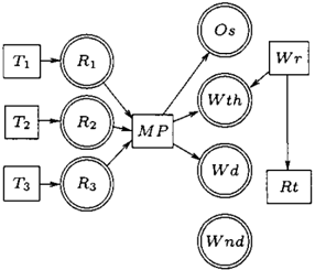
To describe the decision scenario for the king, we have to specify which variables are observable. To do so, we let observable chance variables be doubly circled.

This is done in Figure 1.

An unconstrained influence diagram (UID) is a DAG

三

--;

over decision variables ( rectangular shaped ) , chance variables ( circular shaped ) , and utility variables ( dia­ mond shaped ) . Furthermore, utility variables have no children. There are two types of chance variables, ob­ servables ( doubly circled ) and non-observables ( singly circled ) .

The quantitative specification required is similar to the specification for influence diagrams: conditional prob­ abilities and utility functions. We add the convention that each decision variable D has a cost. If this cost only depends on D, it is not represented graphically, and the cost function is attached to D. We say that an UID is instantiated when the structure has been ex­ tended with the required quantitative specifications.

The semantics of an UID is similar to the semantics of IDs. A link into a decision variable represents in­ formational precedence; a link into a chance variable represents causal influence; a link into a utility vari­ able represents functional dependence. We assume no­ forgetting: at each point of the decision process the decision maker knows all previous decisions and ob­ servations.

We add a semantic clarification, which is not necessary for influence diagrams. As the order of observations and decisions is not determined by the structure, it might seem that a descendant of a decision node may be observed prior to the decision. This will have no meaning, and therefore descendants of a decision node should be regarded as non-existing until the decision is made. If you have the option of observing a variable before and after an ancestral decision, this should be modeled through two different variables.

On the other hand, an observable can be observed when all its antecedent decision variables have been decided upon. In that case we say that the observable

is free, and we release an observable when the last de­ cision in its ancestral set is taken.

The structural specification yields a partial temporal order. The temporal order for Figure 1 is shown in Fig­ ure 2.

If the structure is extended to a linear ordering we get an influence diagram. Such an extension is called an admissible order. The problem addressed in Nielsen and Jensen (1999) is whether all admissible orderings yield the same optimal strategy.

When dealing with UIDs, the concept of strategy is more complex then is the case for IDs. In principle we look for a set of rules telling us what to do given the current information, where "what to do" is to choose the next action as well as choosing a decision option if the next action is a decision. Notice that the choice of next action may be dependent on the specific infor­ mation from the past.

Notation Let r be an unconstrained influence dia­ gram. The set of decision variables is denoted Dr, the set of observables is denoted Or. Let X <:;; Dr U Or be a set of variables; sp( X) denotes the set of configu­ rations over X ( ignoring order ) . The partial temporal order induced by r is denoted -<r. When obvious from the context we avoid the subscript.

Definition 1 Let r be an UID.

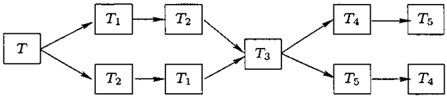
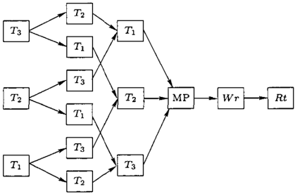
An S-DAG is a directed acyclic graph G. The nodes are labeled with variables from Dr U Or such that each maximal directed path in G represents an admissible ordering of Dr U Or. (Figure 3 gives an example of an S-DAG for the king's problem).

Let N be a node in an S-DAG. The history of N (denoted hst(N)) is the union of labels of N and its ancestors. The union of labels of N 's children is de­ noted ch( N). A step-policy for N is a function a : sp( hst( N)) -> ch(N).

A step-strategy for r is a couple ( L:, S) , where L: is an 8-DA G for r and S is a set of step-policies, one for each node in L:.

A policy for N is an extension of a step-policy , such that whenever the step-policy yields a decision variable D, then the policy yields a state of D . A strategy for r is an 8-D AG together with a policy for each node.

We now need to define the concept of expected utility (EU) of a strategy for UID. As a precise definition is a bit complex we shell not give it here. Instead, notice that any strategy 8 for an UID can be folded out to a strategy tree: following the policies in 8 we construct a tree where all root-leaf paths represent an admissible ordering. The expected utility of a strategy tree is defined as for decision trees, and the expected utility of a strategy is the expected utility of the corresponding strategy tree.

A solution to an UID is a strategy of maximal EU. Such a strategy is called optimal.

3 Normal form S-DAGs

We wish to construct an S-DAG which is guaranteed to contain an S-DAG for an optimal strategy. Our con­ cern is to construct it as small as possible. To reduce the S-DAG we use the following two observations

1. The expected utility can never increase by delay­ ing an observation 1.

So, we need not have any path with a decision variable placed before a free observation.

1 0bservations are cost free.

1. As two maximizations (summations) over finite variables are commutable, a sequence of variables of the same type can be commuted without chang­ ing the EU. So, a sequence of consecutive vari­ ables of the same type can be characterized as a set rather than a sequence.

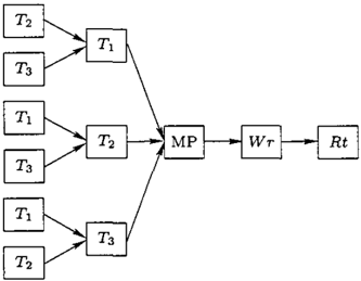
��2--������=�be��� than single variables. When it causes no confusion we will not distinguish between a node and its label, and when the label consists of one variable, we avoid talking about it in set terms. Using 1. we restrict ourselves to S-DAGs in normal form: each parent of a node labeled with an observable V contains a decision node D such that D -< V. Furthermore, nodes with identical history have the same children.

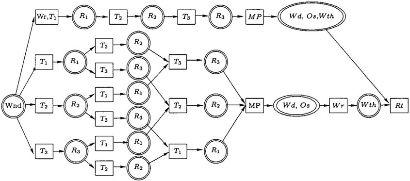
Figure 4 gives a normal form S-DAG for the king's problem.

As the labels of nodes in a normal form S-DAG are sets of variables of the same type, we classify them as decision nodes and observation nodes. Note that an observation node has only decision nodes as children, and a decision node D may have as children either a single observation node 0 or a set of decision nodes. The decision children of D are in the first case the children of 0 and in the latter case the children of D.

Definition 2 The skeleton of a normal form 8-DAG G is a DAG over G 's decision nodes . There is an edge from D to D ' if and only if D ' is a decision child of Din G.

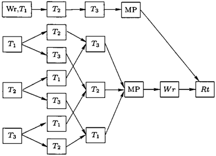
Figure 5 shows the skeleton of the normal form S-DAG in Figure 4. Note that the normal form S-DAG can easily be reconstructed from its skeleton.

三

-;

We aim at constructing a GS-DAG: an S-DAG which is guaranteed to include an S-DAG for an optimal strat­ egy. Due to 1. and 2. we only need to search among normal form S-DAGs.

4 Construction of GS-DAGs

We wish to construct a GS-DAG as small as possible. In this section we present an algorithm exploiting some simple rules reducing the size. In Section 6 we shall present other reduction rules.

Instead of presenting the general algorithm, we shall show how it works in the king's problem. We construct the skeleton of a GS-DAG, and the construction works in reverse temporal order. That is, we start off con­ sidering which decision can be taken last.

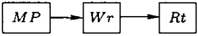
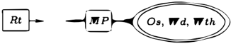
From the partial order in Figure 2 we see that only Rt and M P can be the last decision. Consider the situation where M P is last. Then the observations

{Os, W d, Wt} must follow this decision, and Rt comes before MP. ( See Figure 6)

If the child of Rt is an observation, this observation does not require Rt, and Rt can be moved to the right ( 1. above ) . The same holds if the child of Rt is a decision. So eventually, Rt is the last variable.

In the next step we have to consider W r and M P. For the same reason as above, M P cannot come after W r ( Wr can be commuted with everything except Wth and Rt) . We get the partial skeleton in Figure 7.

Now, we can choose among the Tis, and the skeleton is branched. Figure 8 shows the skeleton after two branchings.

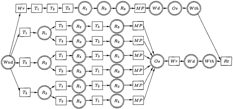
When incorporating the last Ti in the skeleton we no­ tice that some of nodes will have identical history. Therefore, these nodes can be identified. We end up with the skeleton in Figure 10, and with the GS-DAG in Figure 9).

Notation Let G be a partially constructed skeleton for the UID r and letT be a top node of G.

The future ofT is the set of the decision nodes together

with the released observables on the maximal directed paths of G starting in T ( and including T).

The decision variable D in r \ f uture(T) is co-free for T, if all its descendant decision nodes in r are members of the future ofT.

Proposition 4.1 Let D1 and D2 be co-free for the top node T. Let D.( D;) denote the set of observations 0 for which D i -< 0, and which are not members of the future ofT. If D.( D1) c D.( Dz), then Dz shall not be selected as a parent ofT. If D.( D1) = D.( D2) we construct a common parent labeled with D1 and D2.

Proof outline. Assume that D2 is selected. Then, in the eventual GS-DAG D1 is an antecedent of D2. As no observation on any path from D1 to D2 has D1 as an ancestor in the UID, D1 can be commuted with all variables on that path ( including D2). J

Algorithm 1 gives the pseudo code for the construction algorithm. In the pseudo code, every node N in the GS-DAG under construction is uniquely defined by a pair of sets [label(N), f uture(N) \ label(N)]. If a node with the same label and future is already generated, it is re-used instead of generated again.

Algorithm 1 (Generating GS-skeleton)

G � empty graph; process � empty list; free � all decisions without observable descendants (possibly 0); G � add node [free, 0] process � add node [free, 0] while process not empty pNode � take first node from process if exists a decision not in f u t u re( pN o de ) parents� find_parents(pNode) for every parent E parents if node parent does not exist in G create it and add it in process

add link from parent to pNode endfor end while

function find_parents(pNode) for every D � juture(pNode) de(D) <--desc(D)\ juture(pNode) endfor remove all sets de(D) such that there is a D1: de(DJ) c de(D) create sets eq(D) that contains all decisions D1: de(D1) = de(D) return the list of nodes [eq(D),Juture(pNode)]

From the reasoning above we conclude this section with

Proposition 4.2 Algorithm 1 yields a skeleton of the GS-DAG.

5 Solving a GS-DAG

A GS-DAG is solved in almost the same manner as for influence diagrams ( Shachter 1986; Shenoy 1992; Jensen et a!. 1994 ) .

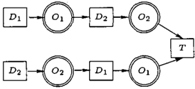
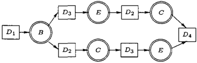
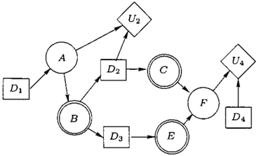
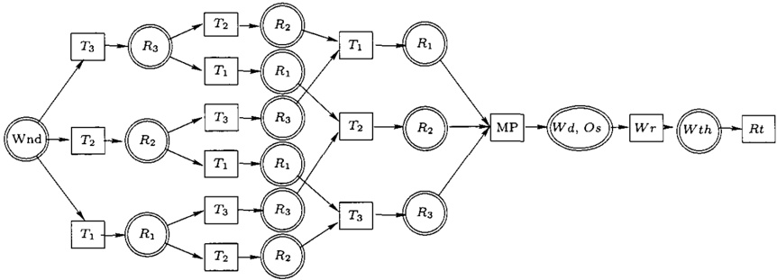
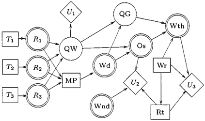
We eliminate variables in reverse order. When a branching point is met, the elimination is branched out, and when several paths meet, the probability po­ tentials are the same, and the utility potentials are uni­ fied through maximization. To illustrate the method we use the UID in Figure 11 with GS-DAG in Fig­ ure 12.

Due to personal biases we illustrate the method us­ ing the lazy propagation method ( Madsen and Jensen 1999 ) . We start off with the two sets

First the non-observables are eliminated. A chance variable X is eliminated in <P by multiplying all potentials with X in the domain to get ¢'x and ( sum ) marginalizing X out of ¢'x to get ¢x. To elimi­ nate X out of Ill we take the sum of all utility poten­ tials with X in the domain, multiply this with ¢'x and marginalize X out. The result is divided by ¢x.

When A and F are eliminated we get the sets

where

Note that Z:pP(FIC, E) is the neutral potential.

We eliminate a decision variable D by taking the sum of the utility potentials with D in the domain and max-marginalizing D out. At the same time, a choice function is determined. When a decision variable is to be eliminated it cannot be in the domain of any probability potential. When D4 has been eliminated we have

Next we branch, and produce one set of potentials after elimination of C and another set after eliminating E.

When eventually D3 has been eliminated in the C­ branch, and D2 is eliminated in theE-branch, we have the two potential sets.

It is no coincidence that the two probability potential sets are identical. They are both the result of sum­ marginalizing the same set of variables from the same set of potentials. As sum-marginalizations can be com­ muted, the two branches must give the same result. Before marginalizing B we unify the utility potentials sets by taking the max:

The step function

The book keeping of potentials is rather easy to han­ dle. After an elimination, create a set of new poten­ tials (or scripts for computing them); and for the other potentials, just keep a pointer.

Our implementation was able to solve the king's prob­ lem in 30 seconds. Solving the worst-case2 problem with nine decisions took 8 minutes. For the worst-case problem with ten decisions the GS-DAG was created, but the evaluation of it ran out of memory.

2 The worst case, with no structural constraints in the UID, forces maximal branching of the GS-DAG, i.e. ""'2 IDI nodes. In the worst case, we need to store a full utility table of size ""' 2 IDI in each node, which for our system caused memory overflow for ten decisions.

6 Exploiting irrelevance

As stated already above, the algorithm presented in Section 4 provides a sufficiently "fat" S-DAG. How­ ever, as the solution of a GS-DAG requires heavy ta­ ble operations, we wish to work with a GS-DAG as slim as possible. As the table operations are resource demanding, we can afford to spend rather much time on graph algorithms for trimming the GS-DAG.

Definition 3 Let D be a decision variable in an in­ fluence diagram, and let past( D) be the decisions and observations performed. A variable A E past( D) is structurally relevant for D if there is an instantiation such that the optimal policy for D is a proper function of A. A is irrelevant if it is not structurally relevant.

Various methods for determining structural relevance in influence diagrams have been developed (Shachter 1998; Nielsen and Jensen 1999; Lauritzen and Nilsson 2001). It holds for IDs as well as for UIDs that the sequencing of the past does not matter. However, the sequencing of the future does matter. We shall return to this in section 7.

Let T be a top node in a partially constructed skeleton. Let D1 and D2 be candidates for being parents ofT, and let 0; be the observations released by D;. If, for example, information on { D1, 01} is not relevant for D2, then we need not include D2 as a parent ofT, and the decision D2 can be pushed forward (see Figure 1 3 ) .

This means that we can extend the algorithm such that at each point of adding parents to a top node we an­ alyze for irrelevance. For any candidate D, if another candidate D' together with its released observations are irrelevant for D, then D is not included as a par­ ent. If all candidates are mutually irrelevant we take any of them.

7 Relevance analysis for UIDs

Relevance analysis in UIDs can be performed in much the same way as in Nielsen and Jensen (1999) for PIDs.

Definition 4 (Lauritzen and Nilsson (2001))

"1

三

Let D be the last decision in an influence diagram. A variable A E past( D) is requisite for D if there is a utility node U such that given past ( D ) \ {A} there is an active path3 from A to U and U is a descendant of D.

Proposition 7.1 If A is not requisite forD , then A is irrelevant for D.

An influence diagram is analyzed for irrelevance by starting with the last decision D. Let r eq( D) be the set of requisite variables in past( D). Then D is sub­ stituted by a chance variable with r eq( D) as parents, and in this way we recursively analyze the decision variables in reverse temporal order.

In the case of UIDs, consider a top node T (see Fig­ ure 14). As the future for T may be performed in different orders, we have to analyze them all.

Let r eq1( D), ... , r eqm( D) be the sets of requisite vari­ ables determined for a candidate D. Then the final set is the union of the reqis.

It is up to further research to establish ways of accu­ mulating information in the process such that we only need to visit T's neighbors for the analysis. Also, it should be investigated whether it might be more effi­ cient to use the solution method in Section 5 directly to establish relevance for the instantiated UID.

8 Conclusions

The system was offered to the king, and he decided to retire immediately and hand over the royal decisions to the marvelous sys­ tem with us operating it.

Acknowledgments

We wish to thank the decision support systems group at Aalborg University for fruitful discussions. In par­ ticular, we thank Thomas D. Nielsen for valuable feed­ back. We also thank the authors of the Elvira4 system for providing a basis for our implementation.

3U is not d-separated from A given past(D) \{A}.

4 http:j /leo.ugr.es;-elvira/

References

Covaliu, Z. and R. M. Oliver (1995). Represen­ tation and solution of decision problems using sequential decision diagrams. Management Sci­ ence 41 (12), 1860-1881.

Howard, A. R. and J. E. Matheson (1981). Influ­ ence diagrams. The Principles and Applications of D ecision Analysis 2, 721-762. Strategic Deci­ sion Group.

Jensen, F., F. V. Jensen, and S. L. Dittmer (1994). From influence diagram to junction tree. In Pro­ ceedings of the Fifteenth Conference on Uncer­ tainty in Artificial Intelligence (UAI-1 gg 4) Seat­ tle, WA, San Francisco, CA, pp. 367-373. Mor­ gan Kaufmann Publishers.

Lauritzen, S. and D. Nilsson (2001). Representing and solving decision problems with limited infor­ mation. Management Science 47(9), 1235-51.

Madsen, A. L. and F. V. Jensen (1999). Lazy evalua­ tion of symmetric bayesian decision problems. In Uncertainty in Artificial Intelligence: Proceed­ ings of the Fifteenth Conference (UAI-1 ggg ), San Francisco, CA, pp. 382-390. Morgan Kauf­ mann Publishers.

Nielsen, T. D. and F. V. Jensen (1999). Wellde­ fined decision scenarios. In Uncertainty in A r­ tificial Intelligence: Proceedings of the Fifteenth Conference (UAI-1 ggg ), San Francisco, CA, pp. 502-511. Morgan Kaufmann Publishers.

Nielsen, T. D. and F. V. Jensen (2000). Repre­ senting and solving asymmetric bayesian deci­ sion problems. In Uncertainty in Artificial In­ telligence: Proceedings of the Sixteenth Confer­ ence (UAI-2000}, San Francisco, CA, pp. 416425. Morgan Kaufmann Publishers.

Shachter, R. D. (1986). Evaluating influence dia­ grams. Operations Research 34(6), 871-882.

Shachter, R. D. (1998). Bayes-ball: The rational past time (for determining irrelevance and req­ uisite information in belief networks and influ­ ence diagrams). In Uncertainty in Artificial In­ telligence: Proceedings of the Fourteenth Confer­ ence (UAI-1 g 98}, San Francisco, CA, pp. 480487. Morgan Kaufmann Publishers.

Shenoy, P. P. (1992). Valuation-based systems for Bayesian decision analysis. Operations Re­ search 40( 3), 463-484.

Shenoy, P. P. (2000). Valuation network repre­ sentation and solution of asymmetric decision problems. European Journal of Operational Re­ search 1 21 (3), 579-608.