Value-Directed Belief State Approximation for POMDPs

Pascal Poupart

Department of Computer Science University of British Columbia Vancouver, BC V6T 1Z4 [email protected]

Abstract

We consider the problem belief-state monitoring for the purposes of implementing a policy for a partially-observable Markov decision process (POMDP), specifically how one might approxi­ mate the belief state. Other schemes for belief­ state approximation (e.g., based on minimizing a measure such as KL-divergence between the true and estimated state) are not necessarily appropri­ ate for POMDPs. Instead we propose a frame­ work for analyzing value-directed approximation schemes, where approximation quality is deter­ mined by the expected error in utility rather than by the error in the belief state itself. We propose heuristic methods for finding good projection schemes for belief state estimation-exhibiting anytime characteristics-given a POMDP value function. We also describe several algorithms for constructing bounds on the error in decision qual­ ity (expected utility) associated with acting in ac­ cordance with a given belief state approximation.

1 Introduction

Considerable attention has been devoted to partially­ observable Markov decision processes (POMDPs) [15, 17] as a model for decision-theoretic planning. Their general­ ity allows one to seamlessly model sensor and action uncer­ tainty, uncertainty in the state of knowledge, and multiple objectives [1, 4]. Despite their attractiveness as a concep­ tual model, POMDPs are intractable and have found prac­ tical applicability in only limited special cases.

Much research in AI has been directed at exploiting cer­ tain types of problem structure to enable value functions for POMDPs to be computed more effectively. These primar­ ily consist of methods that use the basic, explicit state-based representation of planning problems [5]. There has, how­ ever, been work on the use of factored representations that resemble classical AI representations, and algorithms for solving POMDPs that exploit this structure [2, 8]. Repre­ sentations such as dynamic Bayes nets (DBNs) [7] are used to represent actions and structured representations of value functions are produced. Such models are important because

Craig Boutilier

Department of Computer Science University of Toronto Toronto, ON M5S 3H5 [email protected] they allow one to deal (potentially) with problems involving a large number of states (exponential in the number of vari­ ables) without explicitly manipulating states, instead rea­ soning directly with the factored representation.

Unfortunately, such representations do not automatically translate into effective policy implementation: given a POMDP value function, one must still maintain a belie f state (or distribution over system states) online in order to implement the policy implicit in the value function. Belief state maintenance, in the worst case, has complexity equal to the size of the state space (exponential in the number of variables), as well. This is typically the case even when the system dynamics can be represented compactly using a DBN, as demonstrated convincingly by Boyen and Koller [3]. Because of this, Boyen and Koller develop an approx­ imation scheme for monitoring dynamical systems (as op­ posed to POMDP policy implementation); intuitively, they show that one can decompose a process along lines sug­ gested by the DBN representation and maintain bounded er­ ror in the estimated belief state. Specifically, they approx­ imate the belief state by projection, breaking the joint dis­ tribution into smaller pieces by marginalization over sub­ sets of variables, effectively discounting certain dependen­ cies among variables.

In this paper, we consider approximate belief state moni­ toring for POMDPs. We assume that a POMDP has been solved and that a value function has been provided to us in a factored form (as we explain below). Our goal is to de­ termine a projection scheme, or decomposition, so that ap­ proximating the belief state using this scheme hinders the ability to implement the optimal policy as little as possible. Our scheme will be quite different from Boyen and Koller's since our aim is not to keep the approximate belief state as "close" to the true belief state as possible (as measured by KL-divergence). Rather we want to ensure that decision quality is sacrificed as little as possible.

In many circumstances, this means that small correlations need to be accounted for, while large correlations can be ignored completely. As an example, one might imagine a process in which two parts are stamped from the same ma­ chine. If the machine has a certain fault, both parts have a high probability of being faulty. Yet if the decisions for subsequent processing of the parts are independent, the fact

that the fault probabilities for the parts are dependent is ir­ relevant. We can thus project our belief state into two inde­ pendent subprocesses with no loss in decision quality. As­ suming the faults are independent causes a large "error" in the belief state; but this has no impact on subsequent deci­ sions or even expected utility assessment. Thus we need not concern ourselves with this "error." In contrast, very small dependencies, when marginalized, may lead to very small "error" in the belief state; yet this small error can have se­ vere consequences on decision quality.

Because of this, while Boyen and Koller's notion of pro­ jection offers a very useful tool for belief state approxima­ tion, the model and analysis they provide cannot be applied usefully to POMDPs. For example, in [14] this model is integrated with a (sampling-based) search tree approach to solving POMDPs. Because the error in decision quality is determined as a function of the worst-case decision quality with respect to actual belief state approximation error, the bounds are unlikely to be useful in practice. We strongly believe estimates of decision quality error should be based on direct information about the value function.

In this paper we provide a theoretical framework for the analysis of value-directed belie f state approximation (VDA) in POMDPs. The framework provides a novel view of ap­ proximation and the errors it induces in decision quality. We use the value function itself to determine which cor­ relations can be "safely" ignored when monitoring one's belief state. Our framework offers methods for bounding (reasonably tightly) the error associated with a given pro­ jection scheme. While these methods are computationally intensive-requiring in the worst case a quadratic increase in the solution time of a POMDP-we argue that this of­ fline effort is worthwhile to enable fast online implemen­ tation of a policy with bounded loss in decision quality. We also suggest a heuristic method for choosing good pro­ jection schemes given the value function associated with a POMDP. Finally, we discuss how our techniques can also be applied to approximation methods other than projection (e.g., aggregation using density trees [ 13]).

2 POMDPs and Belief State Monitoring

2.1 Solving POMDPs

A partially-observable Markov decision process (POMDP) is a general model for decision making under uncertainty. Formally, we require the following components: a finite state space S; a finite action space A; a finite observation space Z; a transition function T : S x A -+ �(S); an observation function 0 : S x A -+ �(Z); and a reward function R : S -+ R.1 Intuitively, the transition function T( s, a) determines a distribution over next states when an agent takes action a in states-we write Pr(s, a, t) to de­ note the probability that state t is reached. This captures un­ certainty in action effects. The observation function reflects the fact that an agent cannot generally determine the true system state with certainty (e.g., due to sensor noise)-we write Pr( s, a, z) to denote the probability that observation z

16-(X) denotes the set of distributions over finite set X.

is made at state s when action a is performed. Finally R( s) denotes the immediate reward associated with s.2

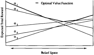
The rewards obtained over time by an agent adopting a spe­ cific course of action can be viewed as random variables R(t) . Our aim is to construct apolicythatmaximizes the ex­ pected sum of discounted rewards E CL�o ··/ R( t)) (where 'Y is a discount factor less than one). It is well-known that an optimal course of action can be determined by consid­ ering the fully-observable belie f state MDP, where belie f states (distributions overS) form states, and a policy rr : �(S) -+A maps belief states into action choices. In prin­ ciple, dynamic programming algorithms for MDPs can be used to solve this problem; but a practical difficulty emerges when one considers that the belief space �(S) is an ISI-1dimensional continuous space. A key result of Sondik [ I7] showed that the value function V for a finite-horizon prob­ lem is piecewise-linear and convex and can be represented as a finite collection of a-vectors.3 Specifically, one can generate a collection N of a-vectors, each of dimension lSI, such that V(b) = ma:xaEN ba. Figure I illustrates a collec­ tion of a-vectors with the upper surface corresponding to V. Furthermore, each a E N has a specific action associ­ ated with it; so given belief state b, the agent should choose the action associated with the maximizing a-vector.

Insight into the nature of POMDP value functions, which will prove critical in the methods we consider in the next section, can be gained by examining Monahan's [15] method for solving POMDPs. Monahan's algorithm pro­ ceeds by producing a sequence of k-stage-to-go value func­ tions Vk, each represented by a set of a-vectors Nk. Each a E Nk denotes the value (as a function of the belief state) of executing a k-step conditional plan. More precisely, let the k-step observation strategies be the set oS< of map­ pings u : Z -+ Nk-l. Then each a-vector in Nk corre­ sponds to the value of executing some action a followed by implementing some u E OSk; that is, it is the value of do­ ing a, and executing the k- 1-step plan associated with the a-vector u( z) if z is observed. Using CP( a) to denote this plan, we have that CP(a) = (a; ifz;, CP(u(z;))'v'z;). We informally write this as (a; u). We write a( (a; u)) to de­ note the a-vector reflecting the value of this plan.

Given Nk, Nk+l is produced in two phases. First, the set of vectors corresponding to all action-observation policies

2 Action costs are ignored to keep the presentation simple.

3 For infinite-horizon problems, a finite collection may not be sufficient [18], but will generally offer a good approximation.

is constructed (i.e., for each a E A and (J' E osk+l, the vector a denoting the value of plan (a, CP((J'(z;) ) ) is added to �k+l ). Second, this set is pruned by removing all domi­ nated vectors. This means that those vectors a such that b·a is not maximal for any belief state b are removed from �k + 1. In Figure 1 , a 4 is dominated, playing no useful role in the representation of V, and can be pruned. Pruning is imple­ mented by a series of linear programs. Refinements of this approach are possible that eliminate (or reduce) the need for pruning by directly identifying only a-vectors that are non­ dominated [17, 6, 4 ]. Other algorithms, such as incremen­ tal pruning [5], are similar in spirit to Monahan's approach, but cleverly avoid enumerating all observation policies. A finite k-stage POMDP can be solved optimally this way and a finite representation of its value function is assured. For infinite-horizon problems, a k-stage solution can be used to approximate the true value function (error bounds can eas­ ily be derived based on the differences between successive value functions).

One difficulty with these classical approaches is the fact that the a-vectors may be difficult to manipulate. A sys­ tem characterized by n random variables has a state space size that is exponential in n. Thus manipulating a single a-vector may be intractable for complex systems. 4 Fortu­ nately, it is often the case that an MDP or POMDP can be specified very compactly by exploiting structure (such as conditional independence among variables) in the system dynamics and reward function [1]. Representations such as dynamic Bayes nets (DBNs) [7 ] can be used to great effect; and schemes have been proposed whereby the a-vectors are computed directly in a factored form by exploiting this rep­ resentation.

Boutilier and Poole [2 ], for example, represent a-vectors as decision trees in implementing Monahan's algorithm. Hansen and Feng [8] use algebraic decision diagrams (ADDs) as their representation in their version of incre­ mental pruning.5 The empirical results in [8 ] suggest that such methods can make reasonably large problems solv­ able. Furthermore, factored representations will likely fa­ cilitate good approximation schemes. There is no reason in principle that the other algorithms mentioned cannot be adapted to factored representations as well.

2.2 Belief State Monitoring

Even if the value function can be constructed in a compact way, the implementation of the optimal policy requires that the agent maintains its belief state over time. The monitor­ ing problem itself is not generally tractable, since each be­ lief state is a vector of size jSj. Given a compact represen­ tation of system dynamics and sensors in the form of DBN, one might expect that monitoring may become tractable us­ ing standard belief net inference schemes. Unfortunately, this is generally not the case. Though variables may be ini-

4 The number of a-vectors can grow exponentially in the worst case, as well; but for many problems the number remains manage­ able; and approximation schemes that simply bound their number have been proposed [6].

5 ADDs, commonly used in verification, have been applied very effectively to the solution of fully-observable MDPs [9].

tially independent (thus admitting a compact representation of a distribution), and though at each time step only a small number of variables become correlated, over time these cor­ relations "bleed through" the DBN, rendering most (if not all) variables dependent after a time. Thus compact repre­ sentation of belief state is typically impossible.

Boyen and Koller [3] have devised a clever approximation scheme for alleviating the computational burden of moni­ toring. In this work, no POMDP is used, but rather a sta­ tionary process, represented in a factored manner (e.g., us­ ing a DBN), is assumed. This might, for example, be the process induced by adopting a fixed policy. Intuitively, they consider projection schemes whereby the joint distribution is approximated by projecting it onto a set of subsets of vari­ ables. It is assumed that these subsets partition the variable set. For each subset, its marginal is computed; the approx­ imate belief state is formed by assuming the subsets are in­ dependent. Thus only variables within the same subset can remain correlated in the approximate belief state. For in­ stance, if there are 4 variables A, B, C and D, the projection scheme { AB, CD} will compute the marginal distributions for AB and CD. The resulting approximate belief state, P(ABCD) = P(AB)P(CD), has a compact, factored representation given by the distribution of each marginal.

Formally, we say a projection scheme S is a set of subsets of the set of state variables such that each state variable is in some subset. This allows marginals with overlapping sub­ sets of variables (e.g., {ABC, BCD}). We view strict par­ titioning as a special type of projection. Some schemes with overlapping subsets may not be computationally useful in practice because it may not be possible to easily generate a joint distribution from them by building a clique tree. We therefore classify as practical those projection schemes for which a joint distribution is easily obtained. Assuming that belief state monitoring is performed using the DBN repre­ senting the system dynamics (see [ 10, 12] for details on in­ ference with DBNs), we obtain belief state bt+l from bt us­ ing the following steps: (a) construct a clique tree encod­ ing the variable dependencies of the system dynamics (for a specific action and observation) and the correlations that have been preserved by the marginals representing bt; (b) initialize the clique tree with the transition probabilities, the observation probabilities and the (approximate, factored) joint distribution bt; (c) query the tree to obtain the distribu­ tion b� at the next time step; and (d) project b� according to some practical projection scheme S to obtain the collec­ tion of marginals representing bt+l = S(b�) . The com­ plexity of belief state updating is now exponential only in the size of the largest clique rather than the total number of variables.

Boyen and Koller show how to compute a bound on the KL-divergence of the true and approximate belief states, exploiting the contraction properties of Markov processes (under certain assumptions). But direct translation of these bounds into decision quality error for POMDPs generally yields weak bounds [14 ]. Furthermore, the suggestions made by Boyen and Koller for choosing good projection schemes are designed to minimize KL-divergence, not to minimize error in expected value for a POMDP. For this rea-

son, we are interested in new methods for choosing projec­ tions that are directly influenced by considerations of value and decision quality.

Other belief state approximation schemes can be used for belief state monitoring. For example, aggregation using density trees can provide a means of representing a belief state with many fewer parameters than the full joint. Our model can be applied to such schemes as well.

3 Error Bounds on Approximation Schemes

In this section, we assume that a POMDP has been solved and that its value function has been provided to us. We also assume that some structured technique has been used so that a-vectors representing the value function are struc­ tured [2, 8]. We begin by assuming that we have been given an approximation scheme S for belief state monitoring in a POMDP and derive error bounds associated with acting according to that approximation scheme. We focus primar­ ily on projection, but we will mention how other types of approximation can be fit into our model. We present two techniques for bounding the error for a given approximation scheme and show that the complexity of these algorithms is similar to that of solving the POMDP, with a (multiplica­ tive) overhead factor of 1 � 1 -

3.1 Plan Switching

Implementing the policy for an infinite-horizonPOMDP re­ quires that one maintains a belief state, plugging this into the value function at each step, and executing the action as­ sociated with the maximizing a-vector. When the belief state b is approximated using an approximation scheme S, a suboptimal policy may be implemented since the maxi­ mizing vector for S(b) will be chosen rather than the max­ imizing vector for b. Furthermore this mistaken choice of vectors (hence actions) can be compounded with each fur­ ther approximation at later stages of the process. To bound such error, we first define the notion of plan switching. We phrase our definitions in terms of finite-horizon value func­ tions, introducing the minor variations needed for infinite­ horizon problems later.

Suppose with k stages-to-go, the true belief state, had we monitored accurately to that point, is b. However, due to previous belief state approximations we take our current be­ lief state to be b. Now imagine our approximation scheme has been ap � lied at time k to obtain S(b). Given �k, rep­ resenting V , suppose the maximizing vectors associated

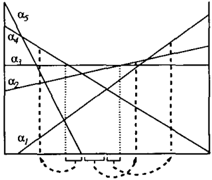
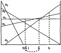
with b, b and S(b) are a1, a2 and aa, respectively (see Fig­ ure 2). The approximation at stage k mistakenly induces the choice of the action associated with a3 instead of a2 at b; this incurs an error in decision quality of b · a2 b · aa. While the optimal choice is in fact a1, the unaccounted er­ ror b · a1 b · a2 induced by the prior approximations will be viewed as caused by the earlier approximations; our goal at this point is simply to consider the error induced by the current approximation.

In order to derive an error bound, we must identify, for each a E �k, the set of vectors Swk (a) that the agent can switch to by approximating its current belief state b given that b identifies a as optimal. Formally, we define

Intuitively, this is the set of vectors we could choose as max­ imizing (thus implementing the corresponding conditional plan) due to belief state approximation. In Figure 3, we see that Swk(aa) = {a1, a2, a4}. The set Swk(a;) can be identified readily by solving a series of O(l�k I) optimiza­ tion problems, each testing the possibility of switching to a specific vector a j E �k, formulated as the following (pos­ sibly nonlinear) program:

The solution to this program has a positive objective func­ tion value whenever there is a belief state b such that a; is optimal at b, and aj is optimal at S(b). Note, in fact, that we need only find a positive feasible solution, not an opti­ mal one, to identify a j as an element of Swk (a;). There are I �k I switch sets to construct, so 0 (I �k 1 2 ) optimization problems need to be solved to determine all switch sets.

For linear approximation schemes (i.e., those in which the constraints on S (b) are linear in the variables b; ), these problems are easily solvable linear programs (LPs). We re­ turn to linear schemes in Section 6. Unfortunately, projec­ tion schemes are nonlinear, making optimization (or iden­ tification of feasible solutions) more difficult. On the other hand, a projection scheme determines a set of linear con­ straints on the approximate belief state S (b). For instance, consider the projection scheme S {CD, DE} for

a POMDP with 3 binary variables. This projection im­ poses one linear constraint on S(b) for each subset of the marginals in the projection:6

Here b' denotes S(b) and b(XY) denotes the cumulative probability (according to belief state b) of all states where X and Y are true. These constraints define an LP that can - k be used to construct a superset Sw (a;) of Swk (a;). Given scheme S = { M 1 , ... , M n}, we define the following LP:

When a feasible positive solution exists, aj is added to the - k set Sw (a;), though in fact, it may not properly be a member of Swk (a;). If no positive solution exists, we know a j - k is not in Swk (a;) and it is not added to Sw (a;). This superset of the switch set can be used to derive an upper bound on error.

While the number of constraints of the type b( M) = b' ( M) is exponential in the size of the largest marginal, we expect that the number of variables in each marginal for a useful projection scheme will be bounded by a small constant. In this way, the number of constraints can be viewed as con­ stant (i.e., independent of state space size).

Though the above LPs (for both linear approximations and projection schemes) look complex, they are in fact very similar in size to the LPs used for dominance testing in Monahan's pruning algorithm and the Witness algorithm, involving O(ISI) variables and O(INk I) constraints. The number of LP variables is exponential in the number of state variables; however, the factored representation of a-vectors allows LPs to be structured in such a way that the state space need not be enumerated (i.e., the variables represent­ ing the state probabilities can be clustered). Precisely the same structuring is suggested in [2] and implemented in [8]. Thus solving an LP to test if the agent can switch from a; to a j has the same complexity as a dominance test in the prun­ ing phase ofPOMDP solving. However, there are O(INk 1 2 ) pairs of a-vectors to test for plan switching whereas the pruning phase may require as few as INk I dominance tests if no vector is pruned. Hence, in the worst case, switch set generation may increase the running time for solving the POMDP by a factor of 0 (INk I) at each stage k.

For a k-stage, finite-horizon POMDP, we can now bound the error in decision quality due to approximationS. Define the bound on the maximum error introduced at each stage j,

6 These equations can be generalized for POMDPs with non­ binary variables, though giving more than one equation per subset.

when a is viewed as optimal, as: 7

Since error at a belief state is simply the expectation of the error at its component states, B1 (a) can be determined by comparing the vectors in S.V j (a) with a component­ wise (with the maximum difference being B1(a)). Let B1 = maxa E Ni B1(a) be the greatest error introduced by a single approximationS at stage j. Then the total er­ ror fork successive approximations is bounded by ug = 2::::7=1 /i B1. For an infinite-horizon POMDP, assume we have been given the infinite-horizon value function N* (i.e. , no stages are involved). Then we only need to compute the switch sets Sw* (a) for this single N-set, and the max­ imum one-shot switching error B'S. The upper bound on the loss incurred by applying s indefinitely is simply u; = B'S /(1 -!). Computing the error u; is roughly equivalent to performing 0( IN* I) dynamic programming backups on N*.

The LP formulation used to construct switch sets is com­ putationally intensive. Other methods can be used how­ ever to construct these switch sets. We have, for example, implemented a scheme whereby belief states are treated as vectors in 3{181, and projection schemes are viewed as dis­ placing these vectors. The displacement vectors (vectors which when added to a belief state b giveS (b)) induced by a scheme S can be computed easily and can be used to deter­ mine the direction in which belief state approximation shifts the true belief state. This is tum can be used to construct overestimates of switch sets. While giving rise to looser er­ ror bounds, this method is much more efficient in practice. Our emphasis, however, is on the analysis of error due to approximation, so we do not dwell on this scheme in this paper (see [ 16] for details).

3.2 Alternative Plans

The cumulative error induced by switching plans at cur­ rent and future stages can be bounded in a tighter way. The idea is to generate the set of alternative plans that may be executed as a result of both current and future approxima­ tions. Suppose that an agent, due to approximation at stage k changes its belief state from b to S(b). This can induce a change in the choice of optimal a-vector in Nk, say from a1 to a2. However, even though the agent has switched and chosen the first action associated with a2, it has not nec­ essarily committed to implementing the entire conditional plan CP( a2) associated with a2. This is because further ap­ proximation at stage k - 1 may cause it to switch from the continuation of CP( a2).

Suppose for instance that CP(a2) = (a;(]"), where (j ( z ) = a3 E Nk- 1 . If z is observed, and the agent updates its (ap­ proximate) belief state S(b) accurately to obtain S(b )',then

7 We use 'S;;,j instead of Sw' to emphasize the fact that we use the approximate switch set generated for a projection scheme; however, all definitions apply equally well to exact switch sets if they are available.

the maximizing vector at the next stage is necessarily a3. But given that S(b)' will be approximated before the max­ imizing vector is chosen, the agent may adopt some other continuation of the plan if a3 does not maximize value for the (second) approximated belief state S(S(b)'). In fact, the agent may implement CP( a4) at stage k 1 for any a4 E Sw k - 1 ( a3). Notice that the value of the plan actually implemented-doing the first action of a2, followed by the first action of a4, and so on-may not be represented by any a-vector in �k.

We can actually construct the values of such plans, and thus obtain much tighter error bounds, while we perform dy­ namic programming. We recursively define the set of al­ ternative sets, or A/t-sets for each vector at each stage.8 We first define

That is, if a is optimal at stage 1 , then any vector in its switch set can have its plan executed. The future alterna­ tive set for any a E �k, where C P ( a ) = (a, a"), is:

If a is in fact chosen to be executed at stage k, true expected value may in fact be given by any vector in FAit (a), this is due to future switching of policies at stages following k. Finally, define

If a is in fact optimal at stage k for a given belief state b, but b is approximated currently and at every future stage, then expected value might be reflected by any vector in Alt (a). These vectors correspond to every possible course of ac­ tion that could be adopted because of approximation: if we switch vectors at stage k, we could begin to execute (the plan associated with) any a' E Sw k (a); and if we begin ex­ ecuting a', we could end up executing (the plan associated with) any a" E FAit (a').

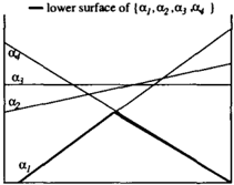
Given these Alt-sets, the error associated with belief state approximation can be given by the maximum difference in value between any a and one of its A/t-vectors. These FAit and A/t-sets can be computed by dynamic programming while a POMDP is being solved. The complexity of this al­ gorithm is virtually identical to that of generating �k from � k - 1, with the proviso that there are l� k l Al t-set s . How­ ever, these sets grow exponentially much like the sets �k would if left unpruned. However, these sets can be pruned in exactly the same way as �-sets, with the exception that since we want to produce a worst-case bound on error, we want to construct a lower surface for the Alt-sets rather than an upper surface.

-Given any Alt-set, we denote by Alt the collection of vectors that are anti-dominating in Alt. For example, if the collec­ tion of vectors in Figure 4, form the set Alt (a), then the vectors a 1 and a4, making up the lower surface of this set,

8 This definition can be more concisely specified, but this for­ mat makes the computational implications clear.

{a 1 ,az,a3 � }

-k -k formAlt (a). FAit (a) is defined similarly. The set of antidominated vectors can be pruned in exactly the same way that dominated a-vectors are pruned from a value function. The same structuring techniques can be used to prevent ex­ � cit state enumeration as well. This pruning can keep the A It-sets very manageable in size. Assuming we have an ap- k proximation Alt (a) of Alt (a) for every a E �k, we con­ -k+1 struct Alt (a) as follows: (a) swk+1 (a) is constructed -k+l for each a E � k+1 ; (b) FAit ( a ) is constructed using -k Alt ( a ) , and is then pruned to retain only anti-dominating -k+l vectors; and (c) Alt (a) is defined as the union of the -k+l k+1 FAit (a') sets for those a' E Sw (a), and is then pruned.

The following quantity bounds the error associated with ap­ proximating belief state using scheme S over the course of a k-stage POMDP, when a represents optimal expected value for the initial belief state:

This error can be computed using simple pointwise com­ parison of a with each such a'. It can also be restricted to that region of belief space where a is optimal; maximizing the difference only over belief states in that area to obtain a tighter bound. Approximation error can be bounded glob­ ally using

Furthermore, E� :::; U� since alternate vectors provide a much tighter way to measure cumulative error.

For an infinite-horizon problem, we can compute switch sets once as in the computation of Us. To compute a tighter bound E'5, we can construct k-stages of Azt-sets, backing up from �·. The bound E� is computed as above, and we set

In this way, we can obtain fairly tight bounds on the error induced by belief state approximation.

4 Value-Directed Approximations

The bounds Bk ( a ) and Ek described above can be used in several ways to determine a good projection scheme. In or­ der to compute error bounds to guide our search for a good

projection scheme, our "generic algorithm" will have to de­ termine the error associated with a different projectionS ap­ plied to each a-vector. Because of this, we will consider the use of dijferent projection schemes So: for each a-vector (at each stage if we have a finite-horizon problem). Despite � he fact that we previously derived bounds on error assurrung a uniform projection scheme, our algorithms work equally well (i.e., provide legitimate bounds) if different projections are used with each vector. The projection So: adopted for vector a simply influences its switch set. Since the agent knows which vector it is "implementing" at any point in time we can record and easily apply the projection scheme So: f � r that vector. This allows the agent to tailor its belief state approximation to provide good results for its currently anticipated course of action. This in tum will lead to much better performance than using a uniform scheme.

4.1 Lattice of Projection Schemes

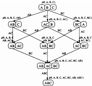
We can structure the search for a projection scheme by con­ sidering the lattice of projection schemes d � fined by � ub­ set inclusion. Specifically, we say St contams S2 (wntten loosely S2 � St) if every subset of S2 . is contai � ed � i . thi � some subset of S1. This means that S2 ts a finer parttt10n than S1. The lattice of projections for three binary variables is illustrated in Figure 5. Each node represents the set of marginals defining some projection S. Above each node, the subsets corresponding to its constraining equations are listed (we refer to each such subset as a constraint). The finest projections (which are the "most approximate" si � ce they assume more independence) are at the top of the latttce. Edges are labeled with the subset of variables correspond­ ing to the single constraining equation th�t � ust be a ? ded to the parent's constraints to obtain the chtld s constramts.

It should be clear that if S2 � St, then St offers (not neces­ sarily strictly) tighter bounds on error when used instead � f S2 at any point. To see this, imagine that various a r proxt­ mation schemes are used for different a-vectors at dtfferent stages, and that S2 is used whenever a E Ni is chosen. If we keep everything fixed but replace S2 with S1 at a, we first observe that Sw�, (a) � Sw�, (a). This ensures that B�, (a) :::; Bt (a) and Bt :::; B�, . If all other projection

. k uk s· . operators are the same, then obvwusly U5 , :::; s , · trrular remarks apply to the infinite-horizon case. Furthermore, given the definition of Alt-sets, reducing the switch set for a at stage k by using S1 instead of S2 ensures that the Alt­ sets at all preceding stages are no larger (and may well be smaller) than they would be if S2 were used. For this rea­ son, we have that E�, :::; E�, (and similarly E5, :::; E5,).

Consequently, as we move down the lattice, the bound on approximation error gets smaller (i.e., our approximations improve, at least in the worst case). Of course, the com­ putational effort of monitoring increases as well. The pre­ cise computational effort of monitoring will depend on the structure of the DBN for the POMDP dynamics and its in­ teraction with the marginals given by the chosen projec­ tion scheme; however, the complexity of inference (i.e., the dominant factors in the corresponding clique tree), can be easily determined for any node in the lattice.

4.2 Search for a Good Projection Scheme

In a POMDP setting, the agent may have a bounded amount of time to make an online decision at each time-step. For this reason, efficient belief-state monitoring is crucial. However, just as solving the POMDP is viewed as an offline operation, so is the search for a good projection sch � me. Thus it will generally pay to expend some computattonal effort to search for a good projection scheme that makes the appropriate tradeoff between decision quality and the complexity of belief state maintenance. For instance, if any scheme S with at most c constraints offers acceptable on­ line performance, then the agent need only search the row of the lattice containing those projection schemes with c con­ straints. However, the size of this row is factorial in c. So instead we use the structure of the lattice to direct our atten­ tion toward reasonable projections.

We describe here a generic, greedy, anytime algorithm for finding a suitable projection scheme. We start with the root, and evaluate each of its children. The child that looks most "promising" is chosen as our current projection scheme. Its children are then evaluated, and so on; this continues un­ til an approximation is found that incurs no err ? r (specifi­ cally, each switch set is a singleton, as we descnbe below), or a bound on the size of the projection is reached. We as­ sume for simplicity that at most c constraints will be al­ lowed. The search proceeds to depth c-n in the lattice and at each node, at most n ( c n) children are evaluated, so a total of 0 ( nc2 - en 2 ) nodes are examined. Since c must be greater than n-the root node itself has n constraints . ­ we assume 0 ( nc2 ) complexity. The structure of the lattice ensures that decision quality (as measured by error bounds) cannot decrease at any step. We note that practical and non­ practical projections are included in the lattice. In figure 5, the only non-practical scheme is S = { AB, AC, B <: }. During the search, it doesn't matter if a node correspondmg to a non-practical scheme is traversed, as long as the final node is practical. If it is not practical, then the best pr�c­ tical sibling of that node is picked or we back . track � nt . tl a practical scheme is found. We also note that smce t � Is � s a greedy approach, we may not discover the bes � � roJectwn with a fixed number of constraints. However, tt t s a well-

structured search space and other search methods for navi­ gating the lattice could be used.

We first describe one instantiation of this algorithm, the finite-horizon U -bound search, for a k-stage, finite-horizon POMDP. Given the collections of a-vectors N i, . . . , Nk, we run the following search independently for each vector a E N' for each i :::; k. The order does not matter; we will end up with a projection scheme S for each a-vector, which is � pplied whenever that a-vector is chosen as optimal at stage z. We essentially minimize (over S) each term B� (a) in � he bound Uk independently. For a given vector a at stage z, the search proceeds from the root in a greedy fashion. Each �hild S of the current node is evaluated by comput­ ing B5 (a), which basically requires that we compute the switch set Sw5 (a), which in turn requires the solution of IN' I LPs. Once the projection schemes S a for each a are fo�nd, the error bound Uk is given by the sum of the bounds B' as described in the previous section. At each stage i, the number of LPs that must be solved is O(nc2IN; 12) since there are O(IN' I) a-vectors and for each a-vector, the lattice search traverses 0 ( nc2) nodes, each requiring the solution of 0( IN' I) LPs. Since the solution of the original POMDP requires the solution of at least INI LPs, the overhead in­ curred is at most a factor of nc21 N 1.

The method above can be streamlined considerably. When comparing two nodes, it is not always necessary to gener­ ate the entire switch set to determine which node has the lowest bound W (a). Each vector a' in a's switch set intro­ duces an error of at most maJQ,{b(aa')}. Since Bi (a) = maxa' ESw ' ( a ) {ma}Q, b(a a')}, we can test vectors a' in decreasing order of contributed error until one vector is found to be in the switch set at one node but not the other. The node that does not include this vector in its switch set � as the lowest bound B� (a) (where S is that node's projec­ twn scheme). Instead of solving IN' I pairs of LPs, generally only a few pairs of LPs will be solved.

When testing whether two different schemes S1 and S 2 allow switching to some a-vector, the LPs to be solved for each scheme are similar, differing only in the con­ straints dictated by each projection scheme. This similarity can be exploited computationally by using techniques that take advantage of the numerous common constraints if we solv � similar LPs "concurrently" (for instance, by solving a stnpped down LP that has only the common constraints and using the dual simplex method to account for the extra constraints). Though details are beyond the scope of this paper, these techniques are faster in practice than solving each LP from scratch. The greedy search can take full ad­ vantage of these speed-ups: each child has only one addi­ tional constraint (compared to its parent), so not only can structure be shared across children, but the parent's solu­ tion can be exploited as well. We reiterate that these LPs can also be structured, so state space enumeration is not re­ quired. Taken together, these computational tricks don't re­ duce the worst-case running time of O(nc2INI2) LPs; how­ ever in practice it is possible that only D(nciNI) LPs need be solved, in which case, when integrated with the algorithm to solve the POMDP, the overhead incurred would be a factor proportional to nc. A thorough experimentation remains to be done.

There are three variations of the algorithm above. The infinite-horizon U -bound algorithm is much like the finite­ horizon version. However, we only have one set of a­ ve � tors, W, rather than k sets. Thus we compute far fewer switch sets, and calculate the final bound using the equation for U*. The finite-horizon E -bound algorithm is similar to the above algorithm as well. The difference is that we com-/ -k pute A _ 1-s � ts (or rather approximations to them, Alt 5 (a)) to obtam tighter bounds on error. To do this requires that we compute the projection schemes for the various stages in order, from the last stage back to the first. Once a good scheme has been found for the elements of N i , the OOt-sets can be computed for stage j + 1 without difficulty (this in­ volves simple DP backups). Then switch sets are computed exactly as above, from whichAzt-sets, and error bounds, are generated. Finally, the infinite-horizon E-bound algorithm � roceeds by computing the switch sets for a given projec­ tion only once for each vector inN*; but additional DP back­ ups to compute Alt-sets (as described in the previous sec­ tion) are needed to derive tight error bounds.

5 Illustrative Example

We describe a very simple POMDP to illustrate the benefits of value-directed approximation, with the aim of demon­ strati � g that minimizing belief state error is not always ap­ propnate when approximate monitoring is used to imple­ ment an optimal policy. The process involves only seven stages with only one or two actions per stage (thus at some stages no choice needs to be made), and no observations are involved. Yet even such a simple system shows the benefits of allowing the value function to influence the choice of ap­ proximation scheme.

We suppose there is a seven-stage manufacturing process whereby four parts are produced using three machines, M, Ml, and M2. Parts PI, P2, P3, and P4 are each stamped in turn by machine M. Once stamped, parts P 1 and P2 are processed separately (in turn) on machine Ml, while parts P3 and P4 are processed together on M2. Machine M may be faulty (FM), with prior probability P r(FM). When the parts are stamped by M, parts P 1 and P2 may be­ come faulty (F 1, F2), with higher probability of fault if FM hol � s. � arts _ P3 and P4 may also become faulty (F3, F4), agam With higher probability if FM; but F3 and F4 are both less sensitive to FM than Fl and F2 (e.g., Pr(FIIFM) = Pr(F2IFM) > Pr ( F3 I F M ) = Pr ( F4 I F M ) ). If PI or P2 are p rocessed on machine M 1 when faulty, a cost is incurred; � f processed when OK, a gain is had; if not processed (re­ Jected), . n � cost or gain is had. When P3 and P4 are pro­ cessed (jomtly)on M3, a greater gain is had if both parts are OK, a lesser gain is had when one part is OK, and a drastic � ost is incurred if both parts are faulty (e.g., machine M3 iS destroyed). The specific problem parameters are given in Table 1.

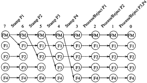
Figure 6 shows the dependencies between variables for the

2000

Table 1: POMDP specifications for the factory example

Stages to go	Actions	Transitions	Rewards
7) StampPI	StampPI	onlyaffects Fl if FM at previous step thenPr(FI) = 0.8 else Pr(FI) = 0.1	no reward
6) StampP2	Stamp P2	only affects F2 if FM at previous step thenPr(F2) = 0.8 elsePr(F2) = 0.1	no reward
5) StampP3	StampP3	only affects F3: if FM at previous step then Pr(F3) = 0.1 elsePr(F3) = 0.05	no reward
4) SlampP4	StampP4	only affects F4: if FM at previous step thenPr(F4) = 0.1 else Pr(F4) = 0.05	no reward
3) Process/RejectPI	ProcessPI RejectPI	all variables are persistant all variables are persistant	if Fl then 0 else 8 4 for every state
2)Process/RejectP2	Process P2 Reject P2	all variables are persistant all variables are persistant	if F2 then 0 else 8 4 for every state
I)Process/RejectP3,P4	ProcessP3,P4	all variables are persistant	if F3 &F4then - 2000 if -F3 &-F4then 16 otherwise 8
	RejectP3,P4	all variables are persistant	3.3 for every state

seven-stage DBN of the example. 9 It is clear with three stages to go, all the variables are correlated. If approximate belief state monitoring is required for execution of the op­ timal policy (admittedly unlikely for such a simple prob­ lem!), a suitable projection scheme could be used.

Notice that the decisions to process P 1 and P2 at stages-to­ go 3 and 2 are independent: they depend only on Pr(Fl) and Pr(F2), respectively, but not on the correlation be­ tween the two variables. Thus, though these become quite strongly correlated with five stages to go, this correlation can be ignored without any impact on the decision one would make at those points. Conversely, F3 and F4 become much more weakly correlated with three stages to go; but the optimal decision at the final stage does depend on their joint probability. Were we to ignore this weak correlation, we run the risk of acting suboptimally.

We ran the greedy search algorithm of Section 4.2 and, as expected, it suggested projection schemes that break all cor­ relations except for FM and F3 with four stages to go, and F3 and F4 with three, two, and one stage(s) to go. The lat­ ter, Pr(F3, F4), is clearly needed (at least for certain prior probabilities on FM) to make the correct decision at the fi-

9 We have imposed certain constraints on actions to keep the problem simple; with the addition of several variables, the prob­ lem could easily be formulated as a "true" DBN with identical dy­ namics and action choices at each time slice.

Table 2: Comparison of different distance measures

Correlation			KL	Loss
FI(F2	0.7704	0.3092	0.4325	1.0
F3/F4	0.9451	0.3442	0.5599	0.0

nal stage; and the former, Pr(FM, F3), is needed to accu­ rately assess Pr(F3, F4) at the subsequent stage. Thus we maintain an approximate belief state with marginals involv­ ing no more than two variables, yet we are assured of acting optimally.

In contrast, if one chooses a projection scheme for this problem by minimizing KL-divergence, L1-distance, or Lz-distance, different correlations will generally be pre­ served. For instance, assuming a uniform prior over FM (i.e., machine M is faulty with probability 0.5), Table 5 shows the approximation error that is incurred according to each such measure when only the correlation between F 1 and F2 is maintained or when only the correlation be­ tween F3 and F4 is maintained. All of these "direct" mea­ sures of belief state error prefer the former. However, the loss in expected value due to the former belief state approx­ imation is 1 .0, whereas no loss is incurred using the lat­ ter. To test this further, we also compared the approxima­ tion preferred using these measures over 1000 (uniformly) randomly-generated prior distributions. If only the F 1 j F2correlation is preserved at the first stage, then in 520 in­ stances a non-optimal action is executed with an average loss of 0.6858. This clearly demonstrates the advantage of using a value-directed method to choose good approxima­ tion schemes.

6 Framework Extensions

The methods described above provide means to analyze value-directed approximations. Though we focused above on projection schemes, approximate monitoring can be ef­ fected by other means. Our framework allows for the anal­ ysis of error of any linear approximation scheme S. In fact, our analysis is better suited to linear approximations: the constraints on the approximate belief state S (b), if linear, allow us to construct exact switch sets Sw( a ) rather than ap­ proximations, providing still tighter bounds.

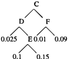
One linear approximation scheme involves the use of den­ sity trees [13]. A density tree represents a distribution by aggregation: the tree splits on variables, and probabilities labeling the leaves denote the probability of every state con­ sistent with the corresponding branch. For instance, the

tree in Figure 7 d�notes a dist_!'ibution over four variables in which states cdef and cdef both have probability 0.1. A tree that is polynomially-sized in the number of variables offers an exponential reduction in the number of parameters required to represent a distribution. A belief state can be ap­ proximated by forcing it to fit within a tree of a bounded size (or satisfying other constraints). This approximation can be reconstructed at each stage, just like projection. It is clear that a density tree approximation is linear. Furthermore, the number of constraints and required variables in the LP for computing a switch set is small.

We also hope to extend this framework to analyze sampling methods [11, 1 3, 1 9] . While such schemes are generally an­ alyzed from the point of view of belief-state error, we would like to consider the impact of sampling on decision quality and develop value-directed sampling techniques that mini­ mize this impact.

7 Concluding Remarks

The value-directed approximation analysis we have pre­ sented takes a rather different view of belief state approxi­ mation than that adopted in previous work. Rather than try­ ing to ensure that the approximate belief state is as close as possible to the true belief state, we try to make the approx­ imate belief state induce decisions that are as close as pos­ sible to optimal, given constraints on (say) the size of the belief state clusters we wish to maintain. Our approach re­ mains tractable by exploiting recent results on factored rep­ resentations of value functions.

There are a number of directions in which this research must be taken to verify its practicality. We are currently ex­ perimenting with the four bounding algorithms described in section 4.2. Ultimately, although these algorithms pro­ vide worst-case bounds on the expected error, it is of in­ terest to gain some insight regarding the average error in­ curred in practice. We are also experimenting with other heuristics, such as the the vector-space method mentioned in Section 3 . I , that may provide a tradeoff between the qual­ ity of the error bounds and the efficiency of their compu­ tation. Other directions include the development of online, dynamic choice of projection schemes for use in search-tree approaches to POMDPs (see, e.g., [14]), as well as solving POMDPs in a bounded-optimal way that takes into account the fact that belief state monitoring will be approximate.

Acknowledgements Poupart was supported by NSERC and carried our this research while visiting the University of Toronto. Boutilier was supported by NSERC Research Grant OGP0121843 and IRIS Phase 3 Project BAC.

References

• [ 1 ] Craig Boutilier, Thomas Dean, and Steve Hanks. Deci­ sion theoretic planning: Structural assumptions and compu­ tational leverage. Journal o f Artificial Intelligence Research, 1 1 : 1-94, 1 999.
• Craig Boutilier and David Poole. Computing optimal poli­ cies for partially observable decision processes using com­ pact representations. In Proceedings of the Thirteenth Na-
• tiona[ Con f erence on Artificial Intelligence, pages 1 1 681 175, Portland, OR, 1996.
• Xavier Boyen and Daphne Koller. Tractable inference for complex stochastic processes. In Proceedings o f the Four­ teenth Con f erence on Uncertainty in Artificial Intelligence, pages 33-42, Madison, WI, 1998.
• Anthony R. Cassandra, Leslie Pack Kaelbling, and Michael L. Littman. Acting optimally in partially ob­ servable stochastic domains. In Proceedings o f the T welfth National Con f erence on Artificial Intelligence, pages 10231028, Seattle, 1994.
• Anthony R. Cassandra, Michael L. Littman, and Nevin L. Zhang. Incremental pruning: A simple, fast, exact method for POMDPs. In Proceedings o f the Thirteenth Con f erence on Uncertainty in Artificial Intelligence, pages 54-61, Prov­ idence, RI, 1 997.
• Hsien-Te Cheng. Algorithms f or Partially Observable Markov Decision Processes. PhD thesis, University of British Columbia, Vancouver, 1988.
• Thomas Dean and Keiji Kanazawa. A model for reason­ ing about persistence and causation. Computational Intel­ ligence, 5(3): 142-150, 1989.
• Eric A. Hansen and Zhengzhu Feng. Dynamic programming for POMDPs using a factored state representation. In Pro­ ceedings o f the Fifth International Con f erence on AI Plan­ ning Systems, Breckenridge, CO, 2000. to appear.
• Jesse Hoey, Robert St-Aubin, Alan Hu, and Craig Boutilier. SPUDD: Stochastic planning using decision diagrams. In Proceedings o f the Fifteenth Con f erence on Uncertainty in Artificial Intelligence, pages 279-288, Stockholm, 1999.
• [ 1 0] Cecil Huang and Adnan Darwiche. Inference in belief net­ works: A procedural guide. Approximate Reasoning, 1 1 : 1158, 1994.
• [ 1 1 ] Michael Isard and Andrew Blake. CONDENSATION­ conditional density propagation for visual tracking. Inter­ national Journal o f Computer Vision, 29(1):5-18, 1998.
• [ 1 2] Uffe Kjaerulff. A computational scheme for reasoning in dy­ namic probabilistic networks. In Proceedings o f the Eighth Conf erence on Uncertainty in AI, pages 121-129, Stanford, 1992.
• [ 1 3] Daphne Koller and Raya Fratkina. Using learning for ap­ proximation in stochastic processes. In Proceedings o f the 15th International Conf erence on Machine Learning, pages 287-295, Madison, 1998.
• [ 1 4] David McAllester and Satinder Singh. Approximate plan­ ning for factored POMDPs using belief state simplification. In Proceedings o f the Fifteenth Con f erence on Uncertainty in Artificial Intelligence, pages 409-416, Stockholm, 1999.
• George E. Monahan. A survey of partially observable Markov decision processes: Theory, models and algorithms. Management Science, 28:1-16, 1982.
• [ 1 6] Pascal Poupart and Craig Boutilier. A vector-space analy­ sis of value-directed belief-state approximation. (in prepa­ ration), 2000.
• Richard D. Smallwood and Edward J. Sondik. The optimal control of partially observable Markov processes over a fi­ nite horizon. Operations Research, 21:1071-1088, 1973.
• [ 1 8] Edward J. Sondik. The optimal control of partially observ­ able Markov processes over the infinite horizon: Discounted costs. Operations Research, 26:282-304, 1978.
• Sebastian Thrun. Monte carlo POMDPs. In Proceedings o f Con f erence on Neural I n f ormation Processing Systems, to appear, Denver, 1999.