Contents
1301.2305
Value-Directed Sampling Methods for Monitoring POMDPs
Pascal Poupart
Department of Computer Science University ofToronto Toronto, ON M5S 3H5 ppoupart@cs. toronto. edu
Luis E. Ortiz
Craig Boutilier
Computer Science Department Brown University Providence, RI, USA 02912-1210 leo@cs. brown.edu
Abstract
We consider the problem of approximate belief-state monitoring using particle filtering for the purposes of implementing a policy for a partially observable Markov decision process (POMDP). While particle fil tering has become a widely used tool in AI for monitor ing dynamical systems, rather scant attention has been paid to their use in the context of decision making. As suming the existence of a value function, we derive er ror bounds on decision quality associated with filtering using importance sampling. We also describe an adap tive procedure that can be used to dynamically deter mine the number of samples required to meet specific error bounds. Empirical evidence is offered supporting this technique as a profitable means of directing sam pling effort where it is needed to distinguish policies.
1 Introduction
Considerable attention has been devoted to partially observ able Markov decision processes (POMDPs) [19] as a model for decision-theoretic planning. Their generality allows one to seamlessly model sensor and action uncertainty, uncer tainty in the state of knowledge, and multiple objectives [ 1, 4]. Despite their attractiveness as a conceptual model, POMDPs are intractable a n d have found practical applica bility in only limited special cases.
The predominant approach to the solution of POMDPs in volves generating an optimal or approximate value f unc tion via dynamic progr amm ing: this value function maps belief states (or distributions over system states) into opti mal expected value, and implicitly into an optimal choice of action. Constructing such value functions is computa tionally intractable and much effort has been devoted to de veloping approximation methods or algorithms that exploit specific problem structure. Potentially more troublesome is the problem of belief state monitoring-maintaining a be lief state over time as actions and observations occur so that the optimal action choice can be made. This too is gen erally intractable, since a distribution must be maintained over the set of system states, which has size exponential in the number of system variables. While value function con struction is an offline problem, belief state monitoring must be effected in real time, hence its computational demands
Department of Computer Science University of Toronto Toronto, ON M5S 3H5 cebly@cs. toronto. edu are considerably more pressing.1
One important family of approximate belief state monitor ing methods is the particle filtering or sequential Monte Carlo approach [6, 13]. A belief state is represented by a random sample of system states, drawn from the true state distribution. This set of particles is propagated through the system dynamics and observation models to reflect the sys tem evolution. Such methods have proven quite effective, and have been applied in many areas of AI such as vision [11] and robotics [21].
While playing a large role in AI, the application of particle filters to decision processes has been limited. While Thrun [20] andMcAllester and Singh [14] have considered the use of sampling methods to solve POMDPs, we are unaware of studies using particle filters in the implementation of a POMDP policy. In this paper we examine just this, focus ing on the use of fairly standard importance sampling tech niques. Assuming a POMDP has been solved (i.e., a value function constructed), we derive bounds on the error in de cision quality associated with particle filtering with a given number of samples. These bounds can be used a priori to determine an appropriate sample size, as well as forming the basis of a post hoc error analysis. We also devise an adaptive scheme for dynamic determination of sample size based on the probability of making an (approximately) op timal action choice given the current set of samples at any stage of the process. We note that similar notions have been applied to the problem of influence diagram evaluation by Ortiz and Kaelbling [15] with good results-our approach draws much from this work, though with an emphasis on the sequential nature of the decision problem.
A key motivation for taking a value-directed approach to sampling lies in the fact that monitoring is an online pro cess that must be effected quickly. One might argue that if the state space of a POMDP is large enough to require sampling for monitoring, then its state space is too large to hope to solve the POMDP. To counter this claim, we note first that recent algorithms [2, 9] based on factored repre sentations, such as dynamic Bayes nets (DBNs), can of ten solve POMDPs without explicit state space enumeration and produce reasonably compact value function representa tions. Unfortunately, such representations do not generally
1While techniques exist for generating finite-state controllers for POMDPs, there are still reasons for wanting to use value function-based approaches [ 17}.
translate into effective (exact) belief monitoring schemes [3]. Even in cases where a POMDP must be solved in a traditional "fiat" fashion, we typically have the luxury of compiling a value function offiine. Thus, even for large PO MOPs, we might reasonably expect to have value func· tion information (either exact or approximate) available to direct the monitoring process. The fact that one is able to produce a value function ojfiine does not imply the ability to monitor the process exactly in a timely online fashion.
We overview PO MOPs, structured solution techniques, and monitoring in Section 2. Section 3 describes a basic par ticle filtering scheme for POMDPs and analyzes its error. We also describe a dynamic sample generation scheme that relies on ideas from group sequential sampling. We exam ine this model empirically in Section 4, and conclude with a discussion of future directions.
2 POMDPs and Belief State Monitoring
2.1 Solving POMDPs
A partially observable Markov decision process (POMDP) is a general model for decision making under uncertainty. Formally, we require the following components: a finite state space S; a finite action space A; a finite observation space Z; a transition function T : S x A -t �(S);2 an observation function 0 : S x A -+ l!.(Z); and a reward function R : S -t R. Intuitively, the transition function T(s, a ) determines a distribution over next states when an agent takes action a in states. This captures uncertainty in action effects. The observation function reflects the fact that an agent cannot generally determine the true system state with certainty (e.g., due to sensor noise). Finally R(s) de notes the immediate reward associated with s.
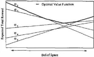
The rewards obtained over time by an agent adopting a spe cific course of action can be viewed as random variables R( t). Our aim is to construct a policy that maximizes the ex pected sum of discounted rewards E(L�o pt R(t)) (where (J is a discount factor less than one). It is well-known that an optimal course of action can be determined by consid· ering the fully observable belief state MDP, where belief states (distributions over S) form states, and a policy rr : l!. ( S) -t A maps belief states into action choices. In prin ciple, dynamic progranuning algorithms for MDPs can be used to solve this problem. A key result of Sondik [ 19] showed that the value function V for a finite-horizon prob· !em is piecewise-linear and convex and can be represented as a finite collection of a-vectors.3 Specifically, one can generate a collection N of a-vectors, each of dimension lSI, such that V(b) = maXaeN ba. Figure 1 illustrates a collec tion of a-vectors with the upper surface corresponding to V. We define ma( b) = arg max,.e � ba to be the maximizing a-vector for belief state b .
Each a E � corresponds to the expected value of executing an implicit conditional plan at a given be lief state. This conditional plan, rr ( a), has the form (a; Ot, 71"1; oz, rrz; · · ·O n , 7r n ), where a is an action, Oi is an
2fl.(X) denotes the set of distributions over finite set X.
3 For infinite-horizon problems, a finite collection may not al ways be sufficient, but will generally offer a good approximation.
observation, and rr; is itself a conditional plan. Intuitively, a plan of this form denotes the performance of action a fol lowed by execution of the remaining plan rr; in response to observation oi. We denote by A(a) the (first) action a of 1r(a). Given belief state b, the agent should execute the action with the maximizing a-vector: A(ma(b)). In deed, if one has access to the entire plan 'IT(ma(b )) , this plan should be executed to termination. We note, however, that the plans 'IT ( cr ) are rarely recorded explicitly.
One difficulty with these classical approaches is the fact that the a-vectors may be difficult to manipulate. A sys tem characterized by n random variables has a state space size that is exponential in n. Thus manipulating a single a-vector may be intractable for complex systems.4 Fortu nately, it is often the case that an MOP or POMDP can be specified very compactly by exploiting structure (such as conditional independence among variables) in the system dynamics and reward function [I]. Representations such as dynamic Bayes nets (DBNs) can be used, and schemes have been proposed whereby the a-vectors are computed directly in a factored form by exploiting this representation.
Boutilier and Poole [2], for example, represent a-vectors as decision trees in implementing Monahan's algorithm. Hansen and Feng [9] use algebraic decision diagrams (ADDs) as their representation in their version of incre mental pruning. The empirical results in [9] suggest that such methods can make reasonably sized problems solv able. Furthermore, factored representations will likely fa cilitate good approximation schemes.
2.2 Belief State Monitoring
Given a value function represented using a collection N of a-vectors, implementation of an optimal policy requires that one maintain a belief state over time in order to ap ply it to N. Given belief state bt at timet, we determine a t = A(ma(bt)), execute a t , make a subsequent obser vation ot· f.l , then update our belief state to obtain b t +l . The process is then repeated. Belief state monitoring is ef fected by computing bt+l = Pr(SW, a t , o t + l ) , which in volves straightforward Bayesian updating. We denote by T(b, a, o ) the update of any belief state b by action a and observation o. We inductively define
___
4 The number of a-vectors can grow exponentially in the worst case, but can often be approximated.
Even if the value function can be constructed in a com pact way, the monitoring problem itself is not generally tractable, since each belief state is a vector of size IS 1. Un fortunately, even using DBNs does not alleviate the diffi culty, since correlations tend to "bleed through" the DBN, rendering most (if not all) variables dependent after a time [3]. Thus compact representation of the exact belief state is typically impossible. Belief state approximation is there fore often required. At any point in time we have an ap proximation (;t of the true belief state bt, and must make our decisions based on this approximate belief state. While sev eral methods for belief state approximation can be used (in cluding projection, aggregation, and variational methods), and important class of techniques for dynamic problems is sampling or simulation methods.
3 Particle Filtering for POMDPs
In this section we examine the impact of particle filtering on decision quality in POMDPs. We first describe a typical sequential importance sampling algorithm, and discuss the use of partial evidence integration (EI) in the DBN to help keep samples on track. We then analyze the error induced by one stage of belief state approximation and show how partial EI allows this analysis to be carried through multiple stages (in a way that is not possible otherwise).
3.1 A Basic Filtering Method for POMDPs
Assume we have been provided with the value function for a specific POMDP M. This value function is represented by a finite collection� of a-vectors. We assume an infinite horizon model so that we have a single set �. We also assume that N is of a manageable size, and that the vec tors themselves are represented compactly (using ADDs, decision trees, linear combinations of basis functions, or some other representation). We emphasize, however, that even if the value function is represented in standard state form, approximate monitoring is often needed. We note that our methods can be applied to approximate value functions, though our analysis assumes an exact set�-
Implementation of the policy induced by this value function requires that a belief state bt be maintained over all times t. At any point in time we assume an approximation bt of the true belief state bt, and make our decisions based on this approximate belief state.
The basic procedure we consider is the use of a particle filter for monitoring, with the approximate belief states so gener ated used for action selection in the POMDP. At any timet, we have a collection bt ofnt weighted particles, or system states, approximating the true distribution bt. Each particle is a pair (s( i ) , w( ;) ). We often simply write s(; ) to refer to the it 11 particle ( i � n t). The total weight of the particle set bt is wt ::: L: w( i) · The particle set b1 represents the following distribution (which we also refer to as bt):
Given this approximation bt of b1, action selection will take
place in the POMDP as if b1 were the true distribution. Thus, we let at = A(ma(b1)), execute action a1, and make observation ot+l. Our new approximate belief state t;t +l is generated by repeating the following steps until nt + I is greater than some desired threshold:
- Draw a state s1 from the distribution b1·
- Draw a state s1+1 from the distribution Pr(st+1ls1 , a1 ) .
- Compute w::: Pr(o1+11st, at, st+l)
- Add sample {s(i)\ w(i)1) ::: {st+ l 1 w) to bt+l and add w to total weight w1·
This sequential importance sampling procedure induces a consistent, though biased, estimate t;t+l of bt+1, and will converge to the true distribution according to the usual con vergence results. The significance of this method lies in the fact that, for a great many systems, it is easy to sample suc cessor states according to the system dynamics (i.e., sample from the conditional distribution in Step 2), and to evaluate the observation probabilities for given states (i.e., compute the weights in Step 3). In contrast, direct computation of Pr(S1+llb 1 , at, o1 +1 ) is generally intractable.
3.2 Evidence Integration
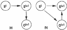
One difficulty with the filtering algorithm above is that the samples generated at time t + 1 are not influenced by ob servation o1 +1, which often allows particles to drift from the true belief state. Since we assume a DBN representa tion of dynamics, partial evidence integration (El) or arc reversal [8] can be used to partially alleviate this problem [13]. The generic structure of a DBN (assuming a fixed ac tion) is shown in Figure 2(a); reversing the arc from St+l to ot+I results in a network shown in Figure 2(b). With this structure, given a particle s( q and observation ot+l, a particles (� 1 can be drawn directly. Of course, the reweighting given ot+l must now be applied to the particles in b1. This gives rise to the following particle filtering procedure used throughout the remainder of the paper:
- (a) Given particle set b1, select action at A(ma(bt)), and observe ot+1 ;
- (b) Reweight samples s(i ) according to Pr( o1+11st, a 1) and normalize to produce i/;
- (c) Draw some number of particles s ( i ) according to l/;
Note that the reweighted distribution // is an approxi mation of Pr( st I a0, · · · at , o1, · · · , o 1 + 1 ) in contrast to b1, which represents Pr(S1 ia0, · · . a1-1, ol, . . . , 01 ).
When the DBN is factored, the arc reversal process can of ten be fairly expensive, since it increases the connectivity of the network. However, the reversal process can take advan tage of the structure in CPTs represented as, say, decision trees or ADD. In this way, the usual exponential increase in table size with the number of added parents is often circum vented [ 5]. We use structured arc reversal techniques in our experiments.
3.3 One-Stage Analysis
As a precursor to bounding the error in decision quality associated with particle filtering, we consider the error in duced by one stage of approximation only (and acting using exact inference at all other stages). We first note the follow ing important fact regarding POMDPs:
Fact 1 Let bt, ll be two belief states s.t. maW) = ma(b1). For any sequence of k observations and actions, let bt+k T(b1,a1 , o1+1 , ···a1+k-l , at+k) an d /;t+k T(l} at ot+l . . ·at+k-1 ot+k) Then ) , ) ' . maW+k) = ma(bHk).
This implies that, if we approximate b1 at timet in such a way that b 1 has the same maximizing a-vector as b1, then we will: (a) choose the correct action at state t; and (b) choose the optimal action at all subsequent stages if we monitor the process exactly (w.r.t. bt) at all subsequent stages.
Now, assume we have been able to exactly compute bt-l, have selected and executed action at-l and made ob servation at. Furthermore, assume that we can com pute Pr(st-1la1-1, d) exactly. With these assumptions, we can sample directly from the distribution b1 T(bt-l, a1-1, o1) using the (arc-reversed) DBN to obtain an u n b i a s e d estimate b1 of bt. We analyze the error associ ated with selecting an a-vector that has maximum expected value w.r.t. b-t and executing its conditional plan to comple tion (or equivalently, acting using exact monitoring from that point on).
Let { s(i)} be a collection ofnt state samples drawn fromb1. The value of any a E N applied to true belief state b1 is:
where a ( s ) denotes the value of a at state s (i.e., the s1h component of a) and Eb' denotes expectation with respect to distribution b1· Thus the value of a can be viewed as a random variable whose expectation (w.r.t. bt) is V�. As such, each term a ( s( i)) is a sample of this random variable and the average of these is an unbiased estimate v� of v�. We can apply (one-sided) Hoeffding bounds to determine the accuracy of this estimate. Specifically:
where R"' is the range of values that can be taken by a (i. e., Ra = maxs{a(s)}- mins{a(s)}).
Given a particular confidence threshold c) and a sample set of size n t we can produce a (one-sided) error bound c:,.. on the accuracy of our estimate v�:
The required sample size given error tolerance c and confi dence threshold 0 for the estimation of v,; is:
We can also bound the simultaneous confidence that each of our e s t i m at es of each a W) has (one-sided) precision£ w ith probability 1J. Decreasing J to 1�1 in Eq. 2 and maximiz ing over all a, we obtain the sample size Nt( c , 8):
Choosing the maximizing a-vector using an approximate l/ with sample size N1 ( c, J) ensures that a 2t-optimal choice is made with probability at least 1o; if the error associated with (arbitrary) nonoptimal behavior is bounded by h, then the one-step approximation error is given by the following:
Theorem 2 If belief state I/ is approximated with Nt ( E' o) particles, with exact monitoring used at all other stages of the process, then the error E (i.e., difference in expected value of the policy implemented and the optimal policy) is bounded by
Here the error incurred is discounted by f3t+l to reflect the fact that the approximation error occurs at stage t of the pro cess. Note that the error h on nonoptimal behavior can be easily bounded (rather loosely) using
though simple domain analysis will generally yield much tighter bounds on h.
One can also perform a post hoc analysis on the choice of a-vector to determine if an optimal c h o i c e has been made with high probability. Assuming n 1 samples have been gen erated, let£ � be the error level determined by Eq. 1 using n t (this is generally tighter than the c used to determine sample size in Eq. 3 since we are looking at a specific vector).
Corollary 3 Let at = ma(bt) and suppose that
Then with probability at least 1 oar-optimal policy will be executed, and our error is bounded by:
二
The parameter T represents the degree to which the value of the second-best a-vector may exceed the value of the best at b1 in the worst-case. Note that this relationship must hold for some T :::; 2£. If the relationship holds forT = 0 (i.e., there is 2£-separation between the maximizing vector and all other vectors at belief state b1) then we are executing the optimal policy with probability at least 1 -o and our error is bounded by j31 + 1oh.
3.4 Multi-stage Analysis
The analysis above assumes that once an a-vector is cho sen, the plan corresponding to that vector will be imple mented over the problem's horizon. In fact, once the first action A (a) is taken, the next action will be dictated by re peating the procedure on the subsequent approximate belief state. Due to further sampling error, the next action cho sen may not be the "correct" continuation of the plan rr( a). Thus we have no assurances that the 2£-optimal policy will be implemented with high probability. In what follows, we assume that our sample size and approximate belief state ll are such that T = 0 at every point in time (i.e., our approx imate beliefs always give at least 2£-separation for the op timal vector). We discuss this assumption further below. We make some preliminary observations and definitions be fore analyzing the accumulated error.
- We first note that b1+ 1 is an unbiased estimate of the distribution T(bt, at, o�+ 1). Though particle filtering does not ensure that b1+1 is unbiased with respect to the true belief state b1+ 1 , our evidence integration pro cedure and reweighting scheme produce "locally" un biased estimates. To see this, notice that the distribu tion// obtained by reweighting b1 w.r.t. o1+1 corre sponds to exact inference assuming the distribution b1 is correct for St. (This exact computation is tractable precisely because of the sparse nature of this approxi mate "prior" on 51.) Thus, the procedure for generat ing samples of st+l using b1 is a simple forward prop agation without reweighting, and thus provides an un biased sample of T (b t , at, o1+1 ) .
- Let us say that a mistake is made at stage t if ma ( b1+ 1) is not optimal w.r.t. T(b1, a1, o1+1 ) . In other words, due to sampling error, the approximate belief state i/+1 differed from the "true" belief state one would have generated using exact inference w.r.t. b1 in such a way as to preclude an optimal policy choice.
We can now analyze the error in decision quality associated with acting under the assumption that T = 0. Let stage t be the first stage at which a mistake is made. If this is the case, we have that ma ( b" + 1 ) = ma ( T ( b" , a", o"+1 ) ) for all k < t. By Fact I , this means that ma(b") = ma(b") for all k < t (where b" is the true stage k belief state one would obtain by exact monitoring). Thus, if stage t is the first stage at which a mistake is made, we have acted ex actly as we would have using exact monitoring for the first t stages of the process. Since our sampling process produces an unbiased estimate b"+1 ofT(b", a", a"+1) at each stage, the probability with which no mistake is made before stage t is at least ( 1 -oj! -t. Assuming a worst-case bound of h on the performance of an incorrect choice (w.r.t. the opti mal policy) at any stage (which is thus independent of any further mistakes being made), we have expected error E on the sampling strategy where N ( o, £) samples are generated at each stage; E is bounded as follows:
Theorem 4
The above reasoning assumes that T reaches zero at each stage of the process, a fact which cannot be assumed a pri ori, since it depends crucially on the particular (approxi mate) belief states that emerge during the monitoring of the process. Unfortunately, strong a priori bounds, as a simple function of£ and J, are not possible if T > 0 at more than one stage. The main reason for this is that the conditional plans that one executes generally do not correspond to a vectors that make up the optimal value function. Specifi cally, when one chooses aT-optimal vector (for some 0 < T $ 2e) at a specific stage, a (worst-case) error ofT is intro duced should this be the only stage at which a suboptimal vector is chosen. If a T-optimal vector is chosen at some later stage ( T > 0), the corresponding policy is r-optimal with respect to a vector that is itself only approximately op timal. Unfortunately, after this second "switch" to a subop timal vector, the error with respect to the original optimal vector cannot be (usefully) bounded using the information at hand.5
However, even without these a priori guarantees on deci sion quality, we expect that in practice, the following ap proximate error bound will work quite well, specifically as a guide to determining appropriate sample complexity, as discussed below:
Intuitively, at each stage of the process a 2e:-optimal vec tor will be chosen with high probability. Though we cannot ensure this, in practice we expect that the cumulative error over those stages where mistakes are not made can be use fully estimated by the first term. The second term accounts for the possibility of mistakes, as in Theorem 4. Here a mis take refers to the probability 1-J event of choosing a vector at a specific stage that is not 2£-optimal.
We also note that a post hoc analysis like that described for one-stage analysis can be used to bound error:
Proposition 5 Let t be the first stage of the process at which T > 0, and t + k be the second such stage. Then
The first term in this bound denotes the error associated with mistakes. The second term reflects the 2e: bound on er5In particular, it is not the case that the error is bounded by 2r [ 17].
ror associated with the first switch to an approximately op timal vector at stage t, while the third reflects the second switch. The main weakness in the bound again lies in this last term and its reliance on h to bound error after a second switch. One way in which these bounds can be strengthened is through the use of switch set analysis, a technique de scribed in [17]. The set of constraints imposed by the sam pling scheme on the true belief state are linear and a priori error bounds can be computed by dynamic programming. Details are beyond the scope of this paper.
3.5 Dynamic Sample Generation
The analysis above allows us to determine a priori the sam ple complexity required to achieve a certain error with a specified probability. Our objective is ultimately to be rea sonably sure we choose the correct (maximizing) cr-vector at each stage of the process. The method above ensures this by requiring that V� is estimated reasonably precisely for each cr. The post hoc analysis of value separation suggests that great precision is not needed if the vectors are widely separated at the true belief state, specifically, if the best vec tor has value much greater than the second best. Draw ing on ideas from the literature on group sequential meth ods [ 12] and multiple-comparisons with the best (MCB) [10] that analyze decision making from this perspective, we describe a method that at each stage generates samples dynamically, using a sampling plan whose termination de pends on results at earlier stages of the plan. The method is inherently simple: we will take samples in batches until we can select an cr-vector satisfying certain requirements. Our method recalls the application of MCB results and group se quential methods by Ortiz and Kaelbling to influence dia grams (see [15] for details and further references).
Suppose we are trying to select the maximizing cr-vector at stage t, using belief state 'bt. The basic structure of our dynamic approach requires that we generate samples from T(6t, at, at+ 1 ) in batches, each of somepredeterminedsize. To generate the jth batch:
- (a) we determine a suitable confidence parameter 8j
- (b) we generate the jth batch of mj samples from T(bt, at' ot+l)
- (c) we compute estimates v� [j] for all vectors cr based on the samples in all j batches, correspond ing precisions E 01 (j], and let crj be the vector with greatest value v� [j]
- (d) we compute threshold -7) = V�. (j) Ea· [j] J J maXa;ta� (V� [j] + E 01 (j]) and terminate if Tj J reaches a certain stopping criterion
We now elaborate on this procedure.
We use MCB results to obtain confidence lower bounds (or one-sided confidence intervals) on the difference in true value between that of the vector with largest value estimate with respect to all the samples in the batches so far and the best of the other vectors. Suppose m1 samples are gener ated in the first batch. Given simultaneous confidence pa rametero1, we obtain the one-sided boundsc:a(j] according to Eq. 1 using 8 = 81/I�XI as the individual confidence pa rameter and nt = m1 as the number of samples. Defining r1 as above, and combining a lower bound for o:i with an upper bound for all the others, we have
If r = r1 is nonpositive, cri is the optimal vector with prob ability at least 1 - o 1. In general, if we stop immediately after processing the first batch and select cri, the error in curred will be at most max(O, r):::; 2C:t = 2 max01 c01[1].
If we are unsatisfied with the precision r achieved, we gen erate a second batch of m2 samples, and propose that
This bound holds if we insist beforehand that we will gen erate the second batch; but it ignores that fact that we gen erate this batch only after realizing our stopping condition was not satisfied using the first batch. This dependence on the bound resulting from the first batch-since these bounds are random variables, this means we do not know a priori whether we will generate a second batch-requires that we correct for multiple looks at the data. We do this by insist ing that both bounds hold jointly, conjoining the bounds ob tained after two batches using the Bonferroni inequality and letting T = m i n { j IJ ::,;2 , a; = a;} Tj:
Hence, if we stop after processing at most 2 batches, then our error in selecting cr; will be at most ma x ( O , r ) with probability at least 1 - (81 + o2). A pp l y i n g this argument up to k batches, we obtain
where r = min{jlj�l<,a j =a:} Tj.
The method as described above will stop at the first batch l such that Tj :::; 0: at this point we are assured of select ing the optimal vector with high probability. If we insist that we force -r to zero, the number of batches k cannot be bounded; thus, we must set the sequence of confidence pa rameters o j such that :Lj: 1 OJ :::; o. For example, we might set 8J = o f(j ( j + 1)) and the individual confidence pa rameters as Oj /llX[. If there is separation between the value of the optimal vector and the second best, the process will stop after a finite number of batches. Hence, we can con tinue the process until -r ::o: 0. However, since the error in the individual estimates decreases only proportionally to J ln j / j, termination might take longer than we wish, de pending on the amount of separation and the vector-value variance. This problem is exacerbated by our use of loose ranges in the computation of the precisions e: a [j].
If we impose a limit B on the number of batches, and want to make sure that our assessment of r holds with proba bility at least 1 -o, we need to set the sequence of confidence parameters OJ such that :L f = 1 OJ :::; o. The easi est way to accomplish our global confidence requirements
二
is to set o i = o /B. Furthermore, if we want to be sure that the method selects a vector with true value that is no less than 2t: from the optimal with the same confidence, then one alternative is to set the number of samples mj in each batch j to the r(maxa R�/(2Be2)) In (BI�I/o)l. If we do not impose specific requirements then the setting of mj is arbitrary, but needs to be fixed in advance. This is because for our analysis to hold, mj cannot depend on the outcomes from the samples themselves. Although arbitrary, in general, the setting of mi should take into consideration a trade-off between reducing the expected total number of samples before the method stop versus reducing the varia tion on the total number of samples.
In general, we expect this method to be effective when there is sufficiently large gap between the best vector and the rest, and/or the ranges in vector values are sufficiently small rel ative to the value separation and the error tolerance. By us ing loose upper bounds on the variances and accuracy pa rameters, the theoretical bounds can become very loose, and hence do not reflect the potential gains we expect. The ver sion presented in this paper is very simple. Many variations on the same idea are possible to try to bring the theoret ical bounds more in accordance with our belief about the expected behavior of the method (for instance, using infor mation about range of differences in value between vector pairs, allocating some samples to estimate variance, etc.), but this is beyond the scope of this paper.
As before, unless we push the error tolerance r to zero at each stage of the monitoring process, we cannot obtain tight bounds on error after that point. However, we can assert:
Theorem 6 Suppose beliefs are monitored according to the dynamic procedure described above using global con fidence parameter o. Furthermore, suppose that r = 0 at each stage. Then error E satisfies
However, as noted above, the computational demands of insisting that r = 0 can be severe if the belief state at some time t is such that little separation exists between the best vector and the second-best (that is, if l} lies close to a "edge" of the value function, where two optimal a-vectors intersect). If r s 0 at all stages up to timet, then the bound described in Proposition 5 holds for this dynamic scheme.
4 Empirical Evaluation
Three test problems were used to carry out experiments test ing the efficacy of our sampling procedures (we refer to [ 16] for the full specification of those problems; see also [18] for a summary). Each of the three problems was solved using Hansen and Feng's [9] ADD implementation of incremental pruning (IP) to produce a set N of a-vectors using a compact ADD representation.
In the following experiments, we report on the use of sam pling for approximate belief state monitoring on three test problems. The goal of the experiments are twofold: to evaluate (i) the impact on decision quality induced by sam pling techniques and (ii) the sample complexity necessary
| Problem | State Space Size | Size ofN | |
| maximum | average | ||
|---|---|---|---|
| o ee | 32 | 102 | 56 |
| Widget | 32 | 205 | 121 |
| Pavement | 128 | 39 | 16 |
to guarantee some level of decision quality. Note that the experiments do not evaluate the running time of sampling methods since that is not the focus of this paper and the ef ficiency gains of such methods have already been clearly demonstrated [II, 21]. In theory, exact monitoring has time complexity on the order ofO{ISI2) whereas sampling has a time complexity in the order ofO(m log lSI) (m is the num ber of samples). Thus, a sampling strategy provides time savings when m < ISI2/log lSI. The reader should also be warned that the scope of the empirical evaluation was limited to test problems for which a set of a-vectors cor responding to an optimal value function can be computed. Hence, as shown in Table 1, lSI and INI are fairly small, and consequently the following experiments should be consid ered preliminary.
The first experiment compares the expected loss incurred by sampling methods to that of a random monitoring ap proach. More precisely, 5000 initial belief states are picked uniformly at random and for each initial belief state, the op timal expected total reward is compared to the cumulative rewards earned by an agent that approximately monitors its belief state over 15 stages. The difference between the opti mal expected total return and the actual return is the loss due to approximate monitoring. Table 2 shows the average loss due to a single approximation at the first stage (assuming exact monitoring for the remaining 14 stages), whereas Ta ble 3 shows the average cumulative loss due to approximate monitoring at each of the 15 stages. When doing random monitoring, the agent picks a belief state at random (uni formly) and executes the optimal action for this random be lief state. This random method can be viewed as a naive strategy that any other approximation method should be able to beat. The sampling methods implemented are basic particle filtering (with partial evidence integration) where a fixed number of particles (20, 40, 80 or 160) are sampled for each approximate belief state. The column "worst" re ports the worst possible expected loss that can be achieved by consistently choosing the worst actions.6 The worst ex pected loss is included to give some idea of the scale of po tential losses due to approximate monitoring.
As expected, the experiments show a gradual decrease in average expected loss as the number of samples increases. When compared to the random strategy (and considering the range of values obtainable across the set of possible be haviors), sampling methods perform quite well. In Table 2,
6 This worst strategy can be computed by minimizing (in stead of maximizing) the expected total reward while solving the POMDP.
| P r ob | Average Single Error Sampling | |||||
|---|---|---|---|---|---|---|
| Rand | Worst | |||||
| 40 | 80 | 160 | ||||
| 1.968 | ||||||
| Prob | Average Cumulative Error | |||||
|---|---|---|---|---|---|---|
| Rand | Sampling | Worst | ||||
| 20 | 40 | 80 | 160 | |||
| Cofi- | 1.653 | 0.100 | 0.043 | 0.018 | 0.017 | 8.014 |
| Widg | 0.109 | 0.098 | 0.069 | 0.045 | 0.022 | 5.778 |
| Pav | 2.319 | 0.124 | 0.072 | 0.045 | 0.024 | 34.24 |
the first row of each problem indicates the actual error in curred and the second row indicates the upper bound 2c pre dicted by the theory (for£ == 0.1). This bound is loose when compared to the actual error due to the worst-case nature of the analysis. The bounds may still provide some guidance regarding the amount of sampling desired to reduce the av erage expected loss to some suitable level (assuming a more or less constant ratio between the bounds and the actual er ror).
In a second experiment, we evaluate the benefits of dynam ically determining the amount of sampling. For given o and (, we evaluate the total number of samples necessary to guarantee that the one-stage sampling error is bounded by 2c with confidence 1 -o. Table 4 shows how this total num ber ()f samples varies as we increase the maximum number of batches. Once again, 5000 random initial belief states are chosen and the average number of samples required to decrease r below 2c is reported. The column for 1 batch corresponds to the standard non-dynamic sampling proce dure. Table 4 reveals that for the widget and pavement prob lems, a dynamic sampling procedure can reduce the sam pling complexity quite dramatically f or a well-chosen max imum number of batches. Unfortunately, the dynamic ap proach does not appear to have offered any savings in the coffee problem. Further investigation is necessary to assess the optimal (maximum) number of batches in general.
In a related paper [18], Poupart and Boutilier also tackle the belief state monitoring problem, but using a vector space method that exploits conditional independence. The idea is to repeatedly approximate belief states using projections as initially proposed by Boyen and Koller [3). Projec tion schemes and sampling approaches diff er in many as pects including the properties of POMDPs for which they
| P r ob | |||||
|---|---|---|---|---|---|
| 1 | 2 | 9 | 10 | ||
| 5 | 254 | 265 | |||
| 139 | 107 | 93 | 78 | 80 | |
| 106 | 64 | 62 | 58 | 59 |
are most suitable. Sampling methods exploit the sparsity of belief distribution whereas projection schemes exploit conditional independence. Given that the coffee, widget and pavement problems are factored POMDPs, the vector space methods tend to perform better than sampling with respect to decision quality. For instance, average losses due to single-stage approximation using the max VS-search method are respectively 0.0013, 0.0082, 0.0014 for the cof f ee, widget and pavement problems; similarly, the average cumulative losses over 15 stages are respectively 0.0154, 0.0519 and 0.0071. However, the computational overhead associated with sampling is minimal while the overhead as sociated with choosing good projection schemes is nontriv ial. We expect the two approaches can be combined in fruit ful ways (as we discuss below).
5 Concluding Remarks
Our value-directed sampling technique can be seen as ap plying methods from the MCB and group sequential sam pling fields to the problem of particle filtering for POMDPs. We are able to derive (worst-case) error bounds on such an approach, and use these bounds to suggest methods to direct sampling in such a way as to choose optimal actions rather than (necessarily) accurately estimate their values. Our ini tial empirical results are encouraging, though clearly much more substantial testing is needed, a task in which we are currently engaged.
This research can be extended in a number of ways in a number of very interesting ways. One important challenge is to provide a stronger analysis of error when the precision p aram eter r > 0. One strategy to circumvent this diffi culty builds on the idea of constructing the set of alternative conditional plans that may be executed when r > 0 [17]. Another challenge is to provide an analysis in the absence of partial EI (which locally removes bias): one idea is to use inf ormation from the DBN parameters to compute a pri ori error bounds; another is to use absolute approximation bounds similar to those used in this paper or optimal rela tive approximation methods to obtain a posteriori bounds on the error tolerance r.
We are very interested in adapting these techniques to other value function representations (e.g., grid-based value func tions) and providing an error analysis of this method when the value function is itself an approximation of the true value function. Finally, previous work using value-directed projection schemes [3, 17] has been used successfully to ex-
:
一
�
ploit the conditional independence present in certain f ac tored POMDPs to speed up belief monitoring. The sam pling approach described in this work does not exploit this type of structure; however, one could sample the variables defining the factored state space in a "stratified" f ashion, or apply Rao-Blackwellisation methods [6, 7].
Acknowledgements: Boutilier and Poupart were sup ported by the Natural Sciences and Engineering Research Council and the Institute for Robotics and Intelligent Sys tems. Ortiz was supported by NSF IGERT award SBR 9870676.
References
- [ 1 ] Craig Boutilier, Thomas Dean, and Steve Hanks. Deci sion theoretic planning: Structural assumptions and compu tational leverage. Journal o f Artificial Intelligence Research, I I : 1 -94, 1 999.
- Craig Boutilier and David Poole. Computing optimal poli cies for partially observable decision processes using com pact representations. In Proceedings o f the Thirteenth Na tional Con f erence on Artificial Intelligence, pages 1 1 681 1 75, Portland, OR, 1 996.
- Xavier Boyen and Daphne Koller. Tractable inference for complex stochastic processes. In Proceedings of the Four teenth Conf erence on Uncertainty in Artificial Intelligence, pages 33-42, Madison, WI, 1998.
- Anthony R. Cassandra, Leslie Pack Kaelbling, and Michael L. Littman. Acting optimally in partially ob servable stochastic domains. In Proceedings o f the T welfth National Con f erence on Artificial Intelligence, pages 1 023-1028, Seattle, 1 994.
- Adrian Y. W. Cheuk and Craig Boutilier. Structured arc re versal and simulation of dynamic probabilistic networks. In Proceedings o f the T hirteenth Con f erence on Uncertainty in Artificial Intelligence, pages 72-79, Providence, Rl, 1 997.
- [6 ] A. Doucet, S. J. Godsill, and C. Andrieu. On sequential monte carlo sampling methods for Bayesian filtering. Statis tics and Computing, 1 0 : 1 97-208, 2000.
- Arnaud Doucet, Nando de Freitas, Kevin Murphy, and Stu art Russell. Rao-Blackwellised particle filtering for dynamic Bayesian networks. In Proceedings o f the Sixteenth Con ference on Uncertainty in Artificial Intelligence, pages 1 761 83, Stanford, 2000.
- Robert Fung and Kuo-Chu Chang. Weighing and integrating evidence for stochastic simulation in Bayesian networks. In Proceedings o f the Fifth Conf erence on U ncertainty in AI, pages 209-219, Windsor, 1 989.
- Eric A. Hansen and Zhengzhu Feng. Dynamic programming for POMDPs using a f actored state representation. In Pro ceedings o f the Fifth I nternational Conf erence on AI Plan ning Systems, Breckenridge, CO, 2000. to appear.
- [ 1 OJ Jason C. Hsu. Multiple Comparisons: Theory and Methods. Chapman and Hall, 1 996.
- [ I I ] Michael Isard and Andrew Blake. CONDENSATION- con ditional density propagation f or visual tracking. Interna tional Journal o f Computer Vision, 29(1):5-18, 1998.
- [ 1 2] Christopher Jennison and Bruce W. Turnbull. Group Sequen tial Methods with Applications to Clinical T rials. Chapman & Hali/CRC, 2000.
- [ 1 3 ] Keiji Kanazawa, Daphne Koller, and Stuart Russell. Stochastic simulation algorithms for dynamic probabilistic networks. In Proceedings of the Eleventh Con f erence on Uncertainty in Artificial Intelligence, pages 346-351, Montreal, 1 995.
- [ 1 4] David McAIIester and Satinder Singh. Approximate plan ning for factored POMDPs using belief state simplification. In Proceedings o f the Fifteenth Con f erence on U ncertainty in Artificial Intelligence, pages 409-416, Stockholm, 1 999.
- [ 1 5] Luis E. Ortiz and Leslie Pack Kaelbling. Sampling methods for action selection in influence diagrams. In Proceedings o f the Seventeenth National Con f erence on Artificial Intelli gence, pages 378-385, Austin, TX, 2000.
- [ 1 6] Pascal Poupart. Approximate value-directed belief state monitoring for partially observable Markov decision pro cesses. Master's thesis, University ofBritish Columbia, Van couver, 2000.
- [ 1 7] Pascal Poupart and Craig Boutilier. Value-directed belief state approximation f or POMDPs. ln Proceedings o f the Six teenth Con f erence on U ncertainty in Artificial Intelligence, pages 497�506, Stanf ord, 2000.
- [ 1 8] Pascal Poupart and Craig Boutilier. Vector-space analysis of belief state approximation for POMDPs. In Proceedings o f the Seventeenth Con f erence on Uncertainty in Artificial In telligence, Seattle, 2001. This Volume.
- [ 1 9] Richard D. Smallwood and Edward J. Sondik. The optimal control of partially observable Markov processes over a fi nite horizon. Operations Research, 2 1 : 1 07 1 - 1 088, 1973.
- Sebastian Thrun. Monte Carlo POMDPs. In Proceedings o f Conf erence on Neural Inf ormation Processing Systems, Denver, 1 999. to appear.
- [21 ] Sebastian Thrun, Dieter Fox, and Wolfram Burgard. A prob abilistic approach to concurrent mapping and localization for mobile robots. Machine Learning, 3 1 :29-53, 1998.