Welldefined Decision Scenarios

Thomas D. Nielsen Finn V. Jensen

Department of Computer Science Aalborg University Fredrik Bayers Vej 7C, DK-9220, Aalborg 0st, Denmark

Abstract

Influence diagrams serve as a powerful tool for modelling symmetric decision problems. When solving an influence diagram we de­ termine a set of strategies for the decisions involved. A strategy for a decision variable is in principle a function over its past. How­ ever, some of the past may be irrelevant for the decision, and for computational reasons it is important not to deal with redundant vari­ ables in the strategies. We show that current methods (e.g. the Decision Bayes-ball algo­ rithm [Shachter, 1998]) do not determine the relevant past, and we present a complete al­ gorithm.

Actually, this paper takes a more general out­ set: When formulating a decision scenario as an influence diagram, a linear temporal or­ dering of the decisions variables is required. This constraint ensures that the decision sce­ nario is well defined. However, the structure of a decision scenario often yields certain de­ cisions conditionally independent, and it is therefore unnecessary to impose a linear tem­ poral ordering on the decisions. In this paper we deal with partial influence diagrams i.e. influence diagrams with only a partial tem­ poral ordering specified. We present a set of conditions which are necessary and sufficient to ensure that a partial influence diagram is welldefined. These conditions are used as a basis for the construction of an algorithm for determining whether or not a partial influ­ ence diagram is welldefined.

1 INTRODUCTION

Graphical modelling for decision support systems is getting more and more widespread. First of all, graph- ical modelling is an appealing way to think of and com­ municate on the underlying structure of the domain in question, but it also helps the modeller to focus on structure rather than calculations. I nfluence diagmms (ID) serve as a powerful modelling tool for symmet­ ric decision problems with several decisions. However, IDs require a linear temporal ordering of the decisions, and this is often felt as an unnecessary constraint. E.g. if no information is gathered between two deci­ sions, then these decisions can be taken independently of each other. This type of very obvious temporal in­ dependence can be handled by a computer system, but temporal independence may be more complicated. For example, observing a variable A immediately before taking a decision D need not have any impact on this particular decision. Hence, we look for an operational characterization of temporal independence in IDs.

The advantages of having an operational charac­ terization of temporal independence are twofold. To take the most obvious advantage first. When a computer system solves an ID it basicly elimi­ nates the variables in reverse temporal order (see [Shachter, 1986], [Shenoy, 1992], [Jensen et al., 1994] and [Zhang, 1998]); eliminating a variable produces a table (function) over all non-eliminated neighbours. However, the reverse temporal order of elimination has a tendency to create very large tables (usually much larger than for Bayesian networks of the same com­ plexity). Thus, if we could relax the temporal order to a partial order, we would have more freedom when looking for a good elimination sequence. To say it an­ other way. When a decision variable D is eliminated we create a strategy for D given its past. If we can reduce the past to contain only the variables required for taking that decision, we have reduced the domain for the strategy function.

The second advantage has to do with the modelling process. That is, will we allow two decisions to be taken independently of each other? Or, do we allow an observation to be made independently of a certain

二

decision? Hence, we work with partial specifications of IDs, and would therefore like to know whether or not this partial structure is ambiguous, and if it is ambigu­ ous we would like the system to give suggestions for further specification of the temporal order. An unam­ biguous partial influence diagram is said to represent a welldefined decision scenario.

In this paper we give · a set of operational rules for determining whether or not a partial influence diagram represents a welldefined decision scenario. These rules are used as a basis for an algorithm for answering this question. The algorithm can furthermore be used in a dialogue between computer and user to pinpoint how to change the model in order to make it unambiguous.

In section 2 we formally introduce IDs, and the terms and notations used throughout this paper. In section 3 we define a partial ID as a generalization of the tradi­ tional ID, and we give a semantic as well as a syntactic characterization of conditions ensuring that a partial influence diagram is unambiguous.

2 INFLUENCE DIAGRAMS

An ID can be seen as a belief network augmented with decision variables and utility functions. Thus, the nodes in the ID can be partitioned into three dis­ joint subsets; chance nodes, decision nodes and value nodes.

The chance nodes (drawn as circles) correspond to chance variables, and represent events which are not under the direct control of the decision maker. The decision nodes (drawn as squares) correspond to deci­ sion variables and represent actions under the direct control of the decision maker. In the remainder of this section we assume a total ordering of the decision nodes, indicating the order in which the decisions are made. 1 Furthermore, we will use the concept of node and variable interchangeably if this does not introduce any inconsistency, and we assume that no barren nodes are specified by the ID since they have no impact on the decisions. 2

The set of value nodes (drawn as diamonds) defines a set of utility functions, indicating the local utility for a given configuration of the variables in their domain. The total utility is the sum or the product of the local utilities; in the remainder of this paper we assume that the total utility is the sum of the local utilities.

1 The ordering of the decision nodes is traditionally rep­ resented by a directed path which includes all decision nodes.

2 A chance node or a decision node is said to be barren if it does not precede any other node, or if all its descendants are barren.

With each chance variable and decision variable X we associate a state space W x which denotes the set of possible outcomes/decision alternatives for X. For a set U' of variables we define the state space as Wu' = x{WxiX E U'}.

The uncertainty associated with each chance variable A is represented by a conditional probability function P(AIPA) : WAuPA -t [0; 1], where PA denotes the immediate predecessors of A.

The arcs in an ID can be partitioned into three dis­ joint subsets, corresponding to the type of node they go into. Arcs into value nodes represent functional dependencies by indicating the domain of the associ­ ated utility function. Arcs into chance nodes, denoted dependency arcs, represent probabilistic dependencies, whereas arcs into decision nodes, denoted informa­ tional arcs, imply information precedence; if there is an arc from a node X to a decision node D then the state of X is known when decision D is made.

Let Uc be the set of chance variables and let Un = { D1, D2, . . . , Dn} be the set of decision variables. As­ suming that the decision variables are ordered by index, the set of informational arcs induces a par­ titioning of Uc into a collection of disjoint subsets C0, C1, . . . , Cn. The set Ci denotes the chance vari­ ables observed between decision Dj and Dj+! thus, the variables in Cj occur as immediate predecessors of Dj+! · This induces a partial order-< on U = Uc UUn i.e. Co -< D1 -< C1 -< · · · -< Dn -< Cn

The set of variables known to the decision maker when deciding on D j is called the informational predeces­ sors of Dj and is denoted pred(Dj). Assuming "no­ forgetting" the set pred(Dj) corresponds to the set of variables that occur before Di under -<. Moreover, based on the "no-forgetting" assumption we can as­ sume that an ID does not specify any redundant no­ forgetting arcs i.e. a chance node can be an immediate predecessor of at most one decision node.

2.1 EVALUATION

When evaluating an ID we identify a strategy for the decision variables; a strategy can be seen as a prescrip­ tion of responses to earlier observations and decisions. The evaluation is usually performed according to the maximum expected utility principle, which states that we should always choose an alternative that maximizes the expected utility.

Definition 1. Let 'I be an ID and let Un denote the decision variables in 'I. A strategy is a set of functions � = {6niD E Un}, where 6n is a decision function given by:

A strategy that maximizes the expected utility is termed an optimal strategy.

In general, the optimal strategy for a decision variable Dk in an ID I is given by:

where pv.+t is the maximum expected utility function for decision Dk+l:

By continuously expanding Equation 1, we get the fol­ lowing expression for the optimal strategy for D k:

where 1/J1, . . . 1/Jl are the utility functions specified by I.

The expression above conveys that the variables are to be eliminated w.r.t. an elimination sequence which is consistent with the partial order, and in what fol­ lows we define a legal elimination sequence as a bijec­ tion a : U B {1, 2, . . . , lUI}, where X -< Y implies a(X) < a(Y). Note that a legal elimination sequence is not necessarily unique, since the chance variables in the sets Ci can be commuted. Even so, any two legal elimination sequences result in the same optimal strategy since the decision variables are ordered totally and 'I:' operations commute; the total ordering of the decision variables ensures that the relative elimination order for any pair of variables of opposite type is in­ variant under the legal elimination sequences (this is needed since a 'max' operation and a 'I:' operation do not commute in general).

3 REPRESENTING DECISION PROBLEMS UNAMBIGUOUSLY

In the section above we described the evaluation of an ID w.r.t. the maximum expected utility principle. The underlying assumption was a total ordering of the decision variables ensuring that the optimal strategy is independent of the legal elimination sequences.

However, it is in general not necessary to have a to­ tal ordering of the decision variables (if ck = 0 then Dk and Dk+1 can be commuted). This can also be seen from the optimal strategy for a decision variable (equation 1), where the elimination order for any two adjacent variables of opposite type may be permuted if the variables do not occur in the same function.

3.1 PARTIAL INFLUENCE DIAGRAMS AND DECISION SCENARIOS

Given that a total ordering of the decision variables may not be needed, we define a partial influence dia­ gram (PID) as a directed acyclic graph consisting of decision nodes, chance nodes and value nodes, assum­ ing that value nodes have no children. Notice, that chance nodes may have several decision nodes as im­ mediate successors, and that no ordering is imposed on the decisions. Additionally, we define a realization of a PID as an attachment of functions to the appropriate variables i.e. the chance variables are associated with conditional probability functions and the value nodes are associated with utility functions.

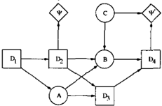
Since the semantics of a PID correspond to the seman­ tics of an ID, a PID induces a partial order -< on the nodes Uc U Uv, as defined by the transitive closure of the following relation (see figure 1):

• Y-< D;, if ( Y ,D;) is a directed arc ini (D; E Uv).
• D; -< Y, if (D;, X1, X2, ... , Xm, Y) is a directed path in I ( Y E Uc U Uv and D; E Uv).
• D; -< A, if A f< Dj for all Di E Uv (A E Uc and D; E Uv).
• D; -< A, if A f< D; and �Di E Uv s.t. D; -< Di and A-< Di (A E Uc and D; E Uv).

In what follows we say that two different nodes X and Y in a PID I are incompatible if X f< Y and Y f< X. Note that a chance node A is incompatible with a de­ cision node D if there exists a decision node D' s.t. D and D' are incompatible and (A, D') is an informa­ tional arc in I and A¢ pred(D)(see figure 1).

As for the traditional ID we seek to identify an opti­ mal strategy when evaluating a PID. Since the optimal strategy for a decision variable may be dependent on variables observed, we define a total order < for a PID.

Definition 2. Let I be a PID and let U = Uv U Uc denote the set of decision variables and chance vari­ ables contained in I. A total ordering of I is a bijec­ tion j3 : U B {1, 2, . . . , lUI}. A total ordering of I is said to be an admissible total ordering if X -< Y im­ plies that j3(X) < j3(Y), where -< is the partial order induced by I.

In what follows <(J will denote the total ordering j3 s.t. X <(! Y if j3(X) < j3(Y) (the index j3 will be

二

一

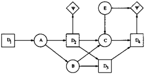
Figure 1: The figure represents a PID which specifies the partial order {B}-< D1-< {E, F,G, D2, D4}-< C4, {B} -< D1-< {E,F} -< D2-< C4, {B} -< D1 -< {G} -< D4 -< C4 and D3 -< C4 (C4 denotes the chance vari­ ables observed (possibly never) after deciding on all the decisions). Thus, D2, D3 and D4 are pairwise in­ compatible, whereas D1 and D4 are not. Furthermore, it can be seen that F is incompatible with D4.

omitted if this does not introduce any confusion). E.g. E < F < D2 < B < D1 < G < D4 < D3 < C4 is a total ordering of the PID in figure 1, but it is not admissible since it contradicts D1 -< D2.

Notice, that an admissible total ordering of a PID I implies that I can be seen as an ID (assuming that redundant no-forgetting arcs have been removed).

Based on the informational predecessors for a decision variable, we define a strategy relative to a total order <, as a set of functions �< = {6.l3!D E Un}, where 613 is a decision function given by:

where pred( D)< = {XIX < D} ( the index < in pred(D)< will be omitted if this does not introduce any confusion). Given a realization of a PID I, we term a strategy relative to <, an optimal strategy rela­ tive to < if the strategy maximizes the expected utility. Likewise we term a decision function 8.!3 contained in an optimal strategy relative to <, an optimal strategy for D relative to <. Note that an optimal strategy for a decision variable D relative to < does not necessar­ ily depend on all the variables observed. Hence we say that an observed variable X is required for D w.r.t. < if there is a realization of I s.t. the optimal strategy for D relative to < is dependent on the state of X.

Since a total order for a PID need not be admissible, we define an admissible optimal strategy for a realiza­ tion of a PID as an optimal strategy relative to an admissible total order.

Definition 3. A realization of a PID I is said to de­ fine a decision scenario if all admissible optimal strate­ gies for I are identical. A PID is said to define a de­ cision scenario if all its realizations define a decision scenario.

The above definition characterizes the class of PIDs which can be considered welldefined, since the set of admissible total orderings for an PID I can be seen as the legal elimination sequences for I (Note that the traditional ID defines a decision scenario). Moreover, in correspondence with the permutations of chance variables in any legal elimination sequence for an ID, we define the following relation for any admissible total order.

Definition 4. Let< be an admissible total order, and let X and Y be two neighbouring variables under <, fulfilling one of the following three conditions:

• X and Y are both chance variables.
• X and Y are both decision variables.
• X and Y are incompatible.

The ordering <1 obtained from < by permuting X and Y according to the rules above is said to be C­ equivalent with<, denoted< =c <1·

Proposition 1. The transitive closure of =c is an equivalence relation.

Theorem 1. All admissible orderings of a partial or­ der -< are C-equivalent.

Proof. It is sufficient to prove the following claim: Let < be an admissible total ordering, and let X and Y be incompatible s.t. X < Y. Then the ordering obtained from < by permuting X and Y is C-equivalent with <.

Assume the claim not to be true. Then there exists an admissible total ordering < and a pair of incompatible variables X, Y which can not be permuted. Let X and Y be such that the segment between X and Y under < is minimal. That is, it is not possible to find any other admissible total order with an incompatible non-permutable pair of variables closer than X andY under<:

Now, start with X and follow < until we reach an in­ compatible variable X;; we know that at least when we reach Y we will meet an incompatible variable. If X; = Y then Y and X;-1 can be permuted, and we have an admissible ordering with an incompatible non­ permutable pair closer than the closest. If i :S n then X and X; are incompatible. If they can not be per­ muted we have a pair of incompatible non-permutable variables closer than the closest. If they can be per­ muted we also obtain a closer pair. 0

So, we are looking for a set of necessary and sufficient conditions ensuring that all admissible orderings yield

the same set of strategies. Actually, we will look for conditions ensuring that orderings, C-equivalent with an admissible ordering, yield the same strategies; this is a bit broader as we allow permutation of two neigh­ bouring decision variables. From Theorem 1 we in­ fer that we can narrow down the scope to neighbour­ ing variables of opposite type (in general neighbour­ ing variables of opposite type can not be permuted without affecting the strategies). Hence, we look for a necessary and sufficient set of conditions granting com­ mutation of two incompatible neighbouring variables of opposite type.

Definition 5. Let I be a PID and let A be a chance variable incompatible with a decision variable D in I. Then A is said to be significant for D if there is a realization and an admissible total order < for I s.t.

• A occurs immediately before D under <.
• The optimal strategy for D relative to < is differ­ ent from the one achieved by permuting A and D in<.

A chance variable is said to be significant for D relative to < if the above conditions are satisfied w.r.t. <.

Notice that if a chance variable A is significant for D w.r.t. < then A is required for D w.r.t. <.

Based on the above definitions we present the following theorem which characterizes the constraints necessary and sufficient for a PID to define a decision scenario.

Theorem 2. The PID I defines a decision scenario if and only if for each decision variable D there does not exist a chance variable A significant for D.

Proof. Follows immediately from Theorem 1 and Def­ inition 5. 0

So, we have reduced the task to the following: Let I be a PID, and let A be a chance variable incompatible with a decision variable D. Is A significant for D?

[Shachter, 1998) presents an algorithm for determining the so called requisite information for a decision vari­ able in an ID. Unfortunately, the algorithm does not meet our needs as shown by the following example.

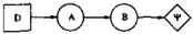
Example 1. When running the algorithm Decision Bayes-ball[Shachter, 1998) on the ID depicted in fig­ ure 2, the chance variable B is marked as requisite for decision D1. However, B is not relevant for the opti­ mal strategy for D1, i.e. the elimination order of B relative to D1 is of no importance when considering the optimal strategy for D1.

0

The following method, which corresponds to itera,. tively replacing decisions by their strategies, has the same drawback. For an ID we start off with the moral graph i.e. informational arcs are removed, undirected arcs are added between nodes with a common child and finally, value nodes are removed together with the directions on the arcs. When eliminating a decision variable D the resulting set of neighbours N (D) is a subset of pred(D). This set of neighbours is invariant w.r.t. the legal elimination sequences, and it is charac­ terized as the set of variables connected in the moral graph to D through a path with no intermediate vari­ able in pred(D). As N(D) contains all the information relevant for determining the optimal strategy for D, it is a candidate for the relevant past. However N(D) may contain variables insignificant for D as can be seen from the ID depicted in Figure 2; B is contained in the neighbouring set for D1 as the elimination of A produces a fill-in between B and D1.

So, neither Decision Bayes-ball nor the elimination method presented above is fine-grained enough to de­ tect all independencies. The problem is that N(D) may contain variables relevant for the maximum ex­ pected utility for D; the maximum expected utility for D may cover utility functions having no influence on the optimal strategy for D. This means that we need to characterize and identify the utility functions on which the optimal strategy for D depends.

Definition 6. The utility function '1/J is relevant for D w.r.t. the admissible total order < for I, if there exists two realizations R1 and R2 of I who only differ on '1/J s.t. the optimal strategies for D relative to < are different in R1 and R2.

We need to determine the structural constraints neces­ sary and sufficient for a utility function to be relevant for a decision variable, and based on this character­ ization we shall define the constraints necessary and sufficient for a chance variable to be significant for a given decision variable.

3.2 RELEVANT UTILITY FUNCTIONS­ EXAMPLES AND RULES

The optimal strategy for a decision variable D is based on the assumption that we always adhere to the max­ imum expected utility principle. Hence, if deciding on D can influence a future decision D' then the utility

二

一

functions relevant for D' may be relevant for D also. From this observation together with the expression for the optimal strategy for D (see equation 1), we present the following metarules. For notational convenience we shall sometimes treat uninstantiated decision nodes as chance nodes with an even prior distribution. More­ over, since a utility function is termed relevant w.r.t. an admissible total order we will mainly consider IDs in the section.

Metarule 1. 1/J is relevant for D in I if there is a real­ ization of I s.t. D has an impact on the expected utility for 7/J.

Metarule 2. 1/J is relevant for D in I if there is a realization of I and a future decision D' s.t. D has an impact on D', for which 1/J is relevant.

Metarule 3. If none of the metarules above can be applied then 1/J is not relevant for D.

The following examples present a set of IDs where we identify the utility functions relevant for a given de­ cision variable. The properties relating to these ex­ amples will be generalized to arbitrary IDs, which will serve as a basis for determining the structural con­ straints necessary for a utility function to be relevant for a given decision variable.

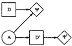
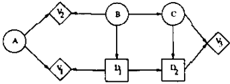
Example 2. Consider the ID depicted in figure 3 and assume that the conditional probability functions are specified s. t. the state of a variable corresponds to the state of its parent.

Figure 3: The figure represents an ID, where the utility function 1/J is relevant for the decision variable D.

It is easy to specify two realizations of 1/J s.t. the op­ timal strategies relative to those realizations differ i.e. 1/J is relevant for D1. 0

Now, assume an arbitrary ID I in which there exists a directed path from a decision node D to a value node 1/J (excluding informational arcs), and assume a realization R of I. Since the conditional probability functions associated with the variables on the path from D to 1/J can be specified s.t. deciding on D has an impact on the expected utility for 1/J, it follows that 1/J is relevant for D.

Rule 1. Let I be a PID, and let f denote I without informational arcs. The utility function 1/J is relevant for the decision variable D if there exists a directed path from D to 1/J in I.

This rule is equivalent to Metarule 1, as can be seen from the mathematical expression correspond­ ing to this metarule: 1/J is relevant for D if

P(dom(7/J)ID, pred(D)) is a function of D, where dom( 1/J) is the chance variables in the domain of '1/J ( uninstantiated decision variables are treated as chance variables). The conditional probability func­ tion P(dom(7/J)Ipred(D), D) is a function of D if D is d-connected to a variable A E dom(¢) given pred(D). However, this implies that there exists a directed path from D to 7/J in f. Conversely, if there exists a di­ rected path from D to 1/J in f, then D is d-connected to a variable A E dom('I/J) given pred(D).

The following examples illustrate, that in order to identify all the utility functions relevant for a given decision variable D, it is in general not sufficient only to consider those utility functions to which there exist a directed path from D.

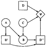
Example 3. When deciding on D4 in the ID depicted in Figure 4 we want to maximize 7/J'. Now, as the deci­ sion variable D2 is d-connected to C given pred(D4), it follows that the decision made w.r.t. D2 may change our belief in C (when deciding on D4) and thereby in­ fluence D4 through 7/J' (D2 is required for D4). Hence '1/J' is relevant for D2, which is also true for 1/J as Dz E dom(7j;). Moreover, knowledge of A may like­ wise change our belief in C when deciding on D4, and since A is influenced by D1 it follows that D1 has an impact on D2 since knowledge of D1 can be taken into account when deciding on D2 (D1 is required for D2). Thus, 7/J' is relevant for both D1 and D2 conveying that '1/J is relevant for D1 also.

This can also be seen by considering the utility func­ tion specified by table 1 together with the functions P(C) = (0, 5; 0, 5), 'I/J1(D2) = (0; 3) and 7f;2(D2) = (3; 0) (we assume that the state of A corresponds to the state of D1 and that P(BID2, A, C) is specified s.t. the state of C is revealed if the state of A, B and D2 are the same, and no knowledge is gained on C if this is not the case).

These functions define two realizations of I who only differ on '1/J, and when evaluating I w.r.t. these real­ izations we obtain two different optimal strategies for D1 i.e. 8n, = d1 if '1/J = '1/JJ and 8n, = d2 if 'ljJ = 'I/J2· From these strategies it can be seen that the utility function 'ljJ influences the optimal strategy for D1 i.e. '1/J is relevant for D1. 0

The example above can be seen as an instance of Metarule 2. Assume an arbitrary ID I and a realiza­ tion of I in which the conditional probability function for any intermediate variable in a converging connec­ tion is as specified in the example above. From this structure we may deduce that, if '1/J' is relevant for a future decision D' and D is required for D', then the utility function '1/J' is relevant for D; D has an impact anD'.

Example 4. When deciding on D4 in the ID depicted in figure 5, we seek to maximize '1/J'. By the arguments given in the example above, it follows that both '1/J and '1/J' are relevant for D2. Additionally, knowledge of B may change our belief in E when deciding on D4, and since B is influenced by A, which in turn is influenced by D1, it follows that D1 has an impact on D2 (A is required for D2). Thus, both 'ljJ and '1/J' are relevant for DJ.

This can also be seen by assuming the two realizations consisting of the utility functions 'I/J1 (D2) = (0; 3) and ?jJ2(D2) = (3; 0) together with functions corresponding to the ones specified in Example 2 and Example 3. When evaluating I w.r.t. these realizations we obtain two optimal strategies which differ on D1 i.e. 8n, = d1 if '1/J = ?/J1 and 8n, = d2 if 'ljJ = ?/J2From these strategies it can be seen that the utility function 'ljJ may influence the optimal strategy for D1 i.e. 'ljJ is relevant for D1. 0

The structural properties relating to the example above can, as for the previous example, be general­ ized to an arbitrary ID. Thus, based on the example above and the deductions made w.r.t. Example 3, we present the following rule.

Rule 2. Let I be a P ID and let < be an admissible total order for I. The utility function 'ljJ is relevant for the decision variable D w. r. t. < if there exists a decision variable D' s. t.

1. D < D' and 'ljJ is relevant forD' w.r.t. <.

ii) either

1. D is required forD' w.r.t. < or
2. there exists a directed path in f from D to a chance variable X E pred(D'), and X is required forD' w.r.t. <.

This rule is equivalent to Metarule 2, since the rule covers all the cases where D can have an impact on a future decision D'; D has an impact on D' if and only if D is required for D' or D influences a variable required for D'.

Note that Rule 2 is not a complete structural rule as it refers to the term "required", which has not yet been characterized structurally. This is done in the following section.

3.3 REQUIRED VARIABLES­ EXAMPLES AND RULES

Having established a method to identify the utility functions relevant for a decision variable, one might think that the required variables could be identified in the following way: Before constructing the moral graph, remove all utility functions not relevant for D and then eliminate the variables as described in Section 3.1. However, the resulting neighbouring set N (D) may still contain variables which are not re­ quired as can be seen from Figure 8: if we add the arc (A, D) and remove the arc (D"','I/J) then A is not required for D but A E N(D) when D is eliminated.

A variable X is required for a decision variable D if X is observed before D and the state of X may influence the optimal strategy for D. Since the optimal strategy for D is dependent on the assumption that we always adhere to the maximum expected utility principle it follows that X is required for D if X has an impact on D or X has an impact on a future decision variable D', on which D also has an impact. Hence, analogously to the metarules specifying the utility functions rele­ vant for a decision variable, we present three metarules concerning the variables required for a given decision variable; according to the definition of a required vari­ able we assume an admissible total order < where a variable X occurs before a decision variable D under <.

Metarule 4. X is required for D if there is a real­ ization s.t. when deciding on D the state of X has an impact on the expected utility for a utility function 'ljJ relevant for D w.r.t. <.

11 4

二

Metarule 5. X is required for D if there is a realiza­ tion and a future decision D' s.t. X has an impact on D', and there exists a utility function 1/J rele­ vant for both D and D' w.r.t. <.

Metarule 6. If none of the metarules above can be applied then X is not required for D.

The following examples present a set of PIDs in which some of the required variables are identified. The prop­ erties described by these examples will be generalized to arbitrary PIDs, and they will serve as a basis for a theorem describing the structural constraints nec­ essary and sufficient for a variable to be required for a given decision variable. In the examples we assume that chance variables, with no immediate predecessors, are given an even prior distribution.

Example 5. Consider the PID I depicted in figure 6. The utility function 1/J is relevant for D for any admis­ sible total ordering of I, and since 1/J is functionally dependent on the chance variable A it follows that A is required for D; as A is incompatible with D there is an admissible total order < with A< D.

0

The example above can be generalized to an arbitrary PID I, assuming that I contains a decision variable D and a variable X. If there exists an admissible total order < s.t. X occurs before D under < and X is d­ connected to a utility function 1/J, relevant for D w.r.t. <, given pred(D), then X is required for D; we can specify a realization of I s.t. the state of X has an impact on the expected utility for 1/J.

Rule 3. Let I be a PID and let D be a decision vari­ able in I. The variable X is required for D if there exists a utility function 1/J relevant forD w.r.t. an ad­ missible total order < s. t. X occurs before D under < and X is d-connected to 1/J given pred(D).

This rule is equivalent to Metarule 4, as can be seen by expressing the metarule mathematically: X is required for D if P(dom( 1/J) [D, pred(D)) is a function of X, and 1/J is a utility function relevant for D. The probability function P(dom('I/J)[D, pred(D)) is a function of X if and only if X is d-connected to 1/J given pred(D).

The following examples show, that in order to identify all the variables required for a decision variable D, it is in general not sufficient only to consider the variables which directly influence the decision made w.r.t. D (see Metarule 5).

Example 6. In the PID I depicted in figure 7 the chance variable A may be observed before D. More­ over, A is required for D" since 1/J is relevant for D" and A is d-connected to 1/J given pred(D"). Now, since 1/J is relevant for D also, it follows that if D < D" then A and D may both have an impact on D". Addition­ ally, if A is observed prior to D then the state of A can be taken into account when deciding on D i.e. A is required for D.

This can also be seen by considering the utility func­ tion specified by Table 2, assuming that P(B[A, C) has the properties of P(C[ D 2, B , E) specified in Ex­ ample 3.

Table 2: The utility function 1/J(D, C, D").

y(D,C, D")	C=C1
D"=d1	C=C2 (10;2) (1; 0)
D"=d2	(0; 1) (2; 10)

The optimal strategy for D relative to A, D , D' ,B, D" ,C is given by 8n(a1) = d2 and 8n(a2) = d1 which indicate, that D is dependent on the state of A (A is required for D). 0

In the example above, the conditional probability func­ tion for B is specified s.t. the state of C is revealed if the state of A corresponds to the state of B, and no knowledge is gained on C if the state of A does not correspond to the state of B. Furthermore, the utility function 1/J relevant for both D and D" is specified s.t. the state of C and the decision made w.r.t. D influ­ ences D". Thus, A is required for D" and therefore required for D also.

Analogously to the previous examples, we may gener­ alize this example by considering an arbitrary PID I and an admissible total order for I, where a variable X occurs before a decision variable D and X is required for a future decision D', which has a relevant utility function in common with D. By specifying the real­ ization of I according to the example above, it follows

that the state of X may influence the decision made w.r.t. D'. Moreover, since D and D' have a relevant utility function in common and X is required for D' we have that X is required for D also; the state of X can be taken into account when deciding on D.

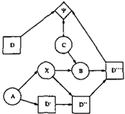
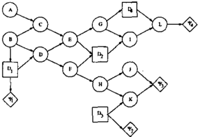
Example 7. Consider the PID I depicted in figure 8. Observing the chance variable A may reveal the state of X, and when deciding on D'" the observation of X may change our belief in the state of C. Now, since '1/J is relevant for both D and Dm the decision made w.r.t. D has an impact on D'", and since the state of A may influence the decision made w.r.t. Dm, and thereby the optimal strategy for D, it follows that the state of A is relevant when deciding on D. That is, A is required for D.

This can also be seen by considering a realiza­ tion of I, where P(X)A) is a deterministic func­ tion and '1/J(D, C, Dm) and P(B)X, C) correspond to '1/J(D, C, D") and P(A ) D 1 , B) respectively (see Ex­ ample 3 and Table 2). When evaluating I w.r.t. A,D,D',X,D",B,Dm,c the optimal strategy for D is given by <lv( ai) = d2 and <lv( a2) = d1 i.e. A is required for D. D

In the example above, the state of X is determined by the state of A, whereas the state of C is determined by the state of X and B i.e. as for the previous examples the state of C is revealed if the state of X corresponds to the state of B, whereas no knowledge is gained on C if the state of X does not correspond to the state of B. Now, consider an arbitrary PID I, and let X denote a variable which occurs before the decision variable D under <, and assume that X is d-connected to a chance variable Y E pred(D') given pred(D). If Y is required for D'(D < D') and D' has a relevant utility function relevant in common with D w.r.t. <,then we can specify a realization, as described in the example above, s.t. the optimal strategy for D is dependent on the state of X. That is, X is required for D.

Rule 4. Let I be a PID and let D be a decision vari­ able in I. Then the variable X is required for D if there exists a utility function '1/J relevant for D w. r. t. an admissible total order <, where X occurs before D and:

1. there exists a decision variable D' (D < D') s.t. '1/J is relevant for D' w.r.t. <.
2. ii) X is required for D' or X is d-connected to a chance variable Y E pred( D') given pred( D) and Y is required for D'.

This rule is equivalent to Metarule 5, since the obser­ vation of X can have an impact on a future decision D' if and only if X is required for D' or X influences a variable required for D'.

The rules 2 and 4 represent a set of simultaneous recur­ sive structural constraints. The recursion terminates because it moves forward in the temporal ordering for each "call".

Based on the rules above we present the following theo­ rem which defines the structural constraints necessary and sufficient for a variable to be required for a given decision variable.

Theorem 3. Let I be an PID and let D be a decision variable in I. Then the variable X is required for D if and only if Rule 3 or Rule 4 (and Rule 1 and Rule 2) can be applied.

Proof. The "if" part of the proof is apparent from the examples above. A mathematial proof of the "only if" part can be performed by closely following the elimi­ nation process when solving an ID. The basic idea is to postpone the calculations until a maximization is performed in order to calculate a strategy for a deci­ sion variable. That is, instead of marginalizing out a chance variable a script is produced, and when maxi­ mizing, the relevant scripts are identified. The details may be found in [Nielsen and Jensen, 1999]. D

Based on the previous rules we present the following rule characterizing the chance variables significant for a given decision variable; this rule is apparent from Rule 3 and Rule 4.

Rule 5. Let I be an PID and let D be a decision vari­ able in I incompatibel with a chance variable A. Then A is significant for D if there exists a utility function '1/J relevant forD w.r.t. an admissible total ordering<, where A occurs immediately before D s.t. :

1. A is d-connected to '1/J given pred(D) or
2. ii) there exists a decision variable D'(D < D') s.t. '1/J is relevant for D' and:
3. A is required for D' or
4. A is d-connected to a chance variable X E pred(D') given pred(D) and X is required for D'.

Additionally we have the folllowing corollaries as a consequence of theorem 3.

Corollary 1. Let I be a PI D and let D be a decision variable in I. Then the utility function '1/J is relevant for D if and only if Rule 1 or Rule 2 can be applied.

Corollary 2. Let I be a PI D and let D be a decision variable in I incompatible with the chance variable A. Then A is significant for D if and only if Rule 5 can be applied.

Corollary 3. Let I be an I D and let D be a decision variable in I. Then X is required for D if and only if Rule 3 or Rule 4 can be applied.

4 ALGORITHMS

In order to determine whether or not a PID defines a decision scenario, it is in principle necessary to inves­ tigate all admissible total orderings < with a pair of incompatible variables being neighbours in <. How­ ever, the set of admissible orderings to investigate can be reduced substantially. E.g. if (A, D) is an incompat­ ible pair, then the ordering of the predecessors is of no importance. Also, if all pairs of incompatible successor nodes have been investigated and found commutably irrelevant, then we can take any admissible order of the successors of A and D. Thus, we start off with maximal pairs of incompatible pairs and work ourself backwards in the partial temporal ordering.

5 CONCLUSION

We have defined a PID as a generalization of the tradi­ tional ID by allowing a non-total ordering of the deci­ sion variables. Because the solution to a decision prob­ lem may be dependent on the temporal ordering of the decisions, we specified the class of PIDs whose solution is independent of the legal evaluation schemes i.e. the class of PIDs that represents a well defined decision sce­ nario. Additionally, we presented the constraints nec­ essary and sufficient for a PID to be contained in this class.

The constraints were given in terms of the concept d-connectivity and are thus readable from the graph­ ical structure. Based on these constraints an algo­ rithm has been designed and implemented to deter­ mine whether or not a PID represents a welldefined decision scenario (the algorithm uses the methods in [ Geiger et a!., 1990] to determine d-connectivity ) . The algorithm has been tested on various PIDs, including those from the paper.

References

[ Geiger et a!., 1990] Geiger, D., Verma, T., and Pearl, J. (1990). d-separation: From theorems to al­ gorithms. Uncertainty in Artificial Intelligence 5, pages 139-149.

[ Jensen et a!., 1994] Jensen, F., Jensen, F. V., and Dittmer, S. L. (1994). From influence diagrams to junction trees. Proceedings of the tenth conference on Uncertainty in Artificial Intelligence, pages 367373.

[ Nielsen and Jensen, 1999] Nielsen, T. D. and Jensen, F. V. (1999). Alternative schemes for the evaluation of influence diagrams. Technical report, Department of Computer Science, Fredrik Bajers 7C, 9220 Aal­ borg, Denmark. To appear.

[ Shachter, 1998] Shachter, R. D. (1998). Bayes ball: The rationale pastime (for determining irrelevance and requisite information in belief networks and influence diagrams. Proceedings of the fourteenth conference on Uncertainty in Artificial Intelligence, pages 480-487.

[ Shachter, 1986] Shachter, R. D. (February 1986). Evaluating influence diagrams. Operations research society of America, 34(6):79-90.

[ Shenoy, 1992] Shenoy, P. P. (1992). Valuation-based systems for Bayesian decision analysis. Operations Research, 40(3):463-484.

[ Zhang, 1998] Zhang, N. L. (1998). Probabilistic infer­ ence in influence diagrams. Proceedings of the four­ teenth conference on Uncertainty in Artificial Intel­ ligence, pages 514-522.